The following object is masked from 'package:terra':

    shift
require(metafor)
Loading required package: metafor
Loading required package: Matrix
Loading required package: metadat
Loading required package: numDeriv
Loading the 'metafor' package (version 4.8-0). For an
introduction to the package please type: help(metafor)
# what rasters are in data rfiles <-list.files('data', pattern ='tif$',full.names =TRUE) rfiles <- rfiles[!grepl('cropland',rfiles)]# read in raster files r.ma <- terra::sds(rfiles)# convert to raster r.ma <- terra::rast(r.ma)# convert rasters to data.table# set first to xy data.frame (NA=FALSE otherwise gridcels are removed) r.df <-as.data.frame(r.ma,xy =TRUE, na.rm =FALSE)# convert to data.table r.dt <-as.data.table(r.df)# setnamessetnames(r.dt,old =c('climate_mat', 'climate_pre','soil_isric_phw_mean_0_5','soil_isric_clay_mean_0_5','soil_isric_soc_mean_0_5','nifert_nfert_nh4','nifert_nfert_no3','nofert_nofert','cropintensity_cropintensity'),new =c('mat','pre','phw','clay','soc','nh4','no3','nam','cropintensity'),skip_absent = T)# select only land area r.dt <- r.dt[!(is.na(mat)|is.na(pre))] r.dt <- r.dt[!(is.na(tillage_RICE) &is.na(tillage_MAIZ) &is.na(tillage_other) &is.na(tillage_wheat))] r.dt <- r.dt[!(is.na(ma_crops_RICE) &is.na(ma_crops_MAIZ) &is.na(ma_crops_other) &is.na(ma_crops_wheat))]# replace area with 0 when missing cols <-colnames(r.dt)[grepl('^ma_|nh4|no3|nam',colnames(r.dt))] r.dt[,c(cols) :=lapply(.SD,function(x) fifelse(is.na(x),0,x)),.SDcols = cols] cols <-colnames(r.dt)[grepl('^tillage',colnames(r.dt))] r.dt[,c(cols) :=lapply(.SD,function(x) fifelse(is.na(x),1,x)),.SDcols = cols] r.dt[is.na(cropintensity), cropintensity :=1]# melt the data.table r.dt.melt <-melt(r.dt,id.vars =c('x','y','mat', 'pre','phw','clay','nh4','no3','nam','soc','cropintensity'),measure=patterns(area="^ma_crops", tillage ="^tillage_"),variable.factor =FALSE,variable.name ='croptype')# set the crop names (be aware, its the order in ma_crops) r.dt.melt[,cropname :=c('rice','maize','other','wheat')[as.numeric(croptype)]]# set names to tillage practices r.dt.melt[, till_name :='conventional'] r.dt.melt[tillage %in%c(3,4,7), till_name :='no-till']# derive the meta-analytical model# read data d1 <- readxl::read_xlsx('Source Data.xlsx',sheet ="FigureS5") d1 <-as.data.table(d1)# add CV for NUE treatment and estimate the SD for missing ones d2<-d1 CV_nuet_bar<-mean(d2$nuet_sd[is.na(d2$nuet_sd)==FALSE]/d2$nuet_mean[is.na(d2$nuet_sd)==FALSE]) d2$nuet_sd[is.na(d2$nuet_sd)==TRUE]<-d2$nuet_mean[is.na(d2$nuet_sd)==TRUE]*1.25*CV_nuet_bar CV_nuec_bar<-mean(d2$nuec_sd[is.na(d2$nuec_sd)==FALSE]/d2$nuec_mean[is.na(d2$nuec_sd)==FALSE]) d2$nuec_sd[is.na(d2$nuec_sd)==TRUE]<-d2$nuec_mean[is.na(d2$nuec_sd)==TRUE]*1.25*CV_nuec_bar# clean up column namessetnames(d2,gsub('\\/','_',gsub(' |\\(|\\)','',colnames(d2))))setnames(d2,tolower(colnames(d2)))# calculate effect size (NUE) es21 <-escalc(measure ="MD", data = d2,m1i = nuet_mean, sd1i = nuet_sd, n1i = replication,m2i = nuec_mean, sd2i = nuec_sd, n2i = replication )# convert to data.tables d02 <-as.data.table(es21)# what are the treatments to be assessed d02.treat <-data.table(treatment =c('ALL',unique(d02$management)))# what are labels d02.treat[treatment=='ALL',desc :='All'] d02.treat[treatment=='EE',desc :='Enhanced Efficiency'] d02.treat[treatment=='CF',desc :='Combined fertilizer'] d02.treat[treatment=='RES',desc :='Residue retention'] d02.treat[treatment=='RFP',desc :='Fertilizer placement'] d02.treat[treatment=='RFR',desc :='Fertilizer rate'] d02.treat[treatment=='ROT',desc :='Crop rotation'] d02.treat[treatment=='RFT',desc :='Fertilizer timing'] d02.treat[treatment=='OF',desc :='Organic fertilizer'] d02.treat[treatment=='RT',desc :='Reduced tillage'] d02.treat[treatment=='NT',desc :='No tillage'] d02.treat[treatment=='CC',desc :='Crop cover']# update the missing values for n_dose and p2o5_dose (as example) d02[is.na(n_dose), n_dose :=median(d02$n_dose,na.rm=TRUE)]# scale the variables to unit variance d02[,clay_scaled :=scale(clay)] d02[,soc_scaled :=scale(soc)] d02[,ph_scaled :=scale(ph)] d02[,mat_scaled :=scale(mat)] d02[,map_scaled :=scale(map)] d02[,n_dose_scaled :=scale(n_dose)]# update the database (it looks like typos) d02[g_crop_type=='marize', g_crop_type :='maize']#Combining different factors d02[tillage=='reduced', tillage :='no-till']# # Combining different factors d02[,fertilizer_type :=factor(fertilizer_type,levels =c('mineral','organic', 'combined','enhanced'))] d02[,fertilizer_strategy :=factor(fertilizer_strategy,levels =c("conventional", "placement","rate","timing"))] d02[,g_crop_type :=factor(g_crop_type,levels =c('maize','wheat','rice'))] d02[,rfp :=fifelse(fertilizer_strategy=='placement','yes','no')] d02[,rft :=fifelse(fertilizer_strategy=='timing','yes','no')] d02[,rfr :=fifelse(fertilizer_strategy=='rate','yes','no')] d02[,ctm :=fifelse(g_crop_type=='maize','yes','no')] d02[,ctw :=fifelse(g_crop_type=='wheat','yes','no')] d02[,ctr :=fifelse(g_crop_type=='rice','yes','no')]#d02[,cto := fifelse(g_crop_type=='other','yes','no')] d02[,ndose2 :=scale(n_dose^2)]# make metafor model m1 <-rma.mv(yi,vi,mods =~fertilizer_type + rfp + rft + rfr + crop_residue + tillage + cover_crop_and_crop_rotation + n_dose_scaled + clay_scaled + ph_scaled + map_scaled + mat_scaled + soc_scaled + n_dose_scaled:soc_scaled + ctm:rfp + ctm + ctw + ctr + ctm:mat_scaled + ndose2 -1,data = d02,random =list(~1|studyid), method="REML",sparse =TRUE)
Warning: Redundant predictors dropped from the model.
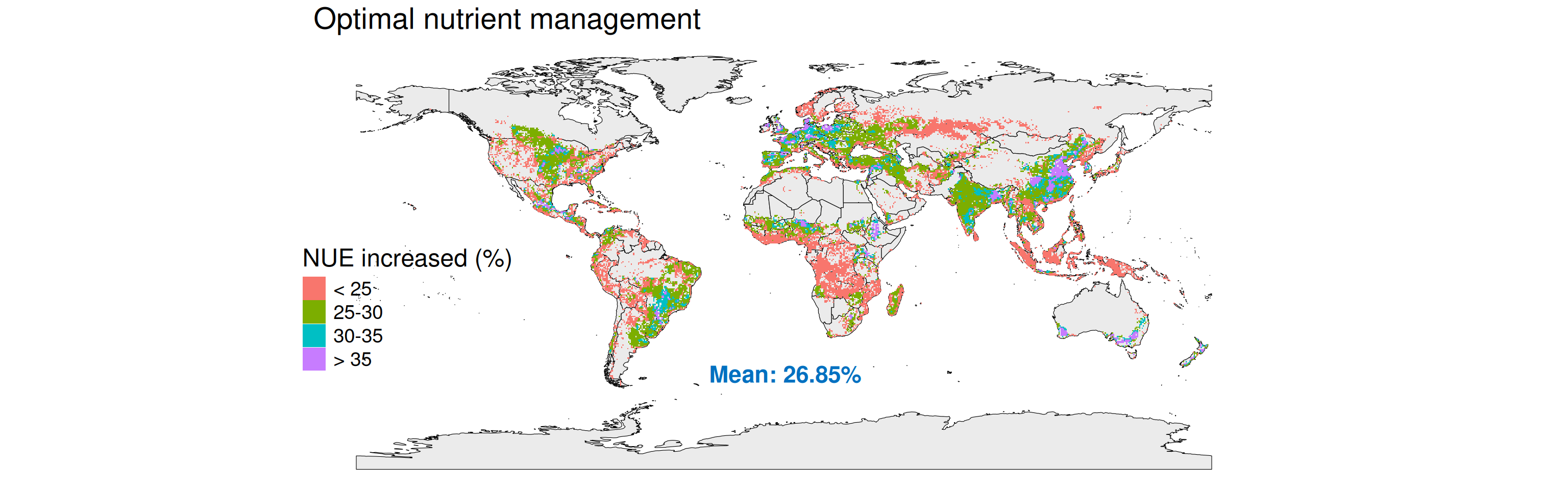
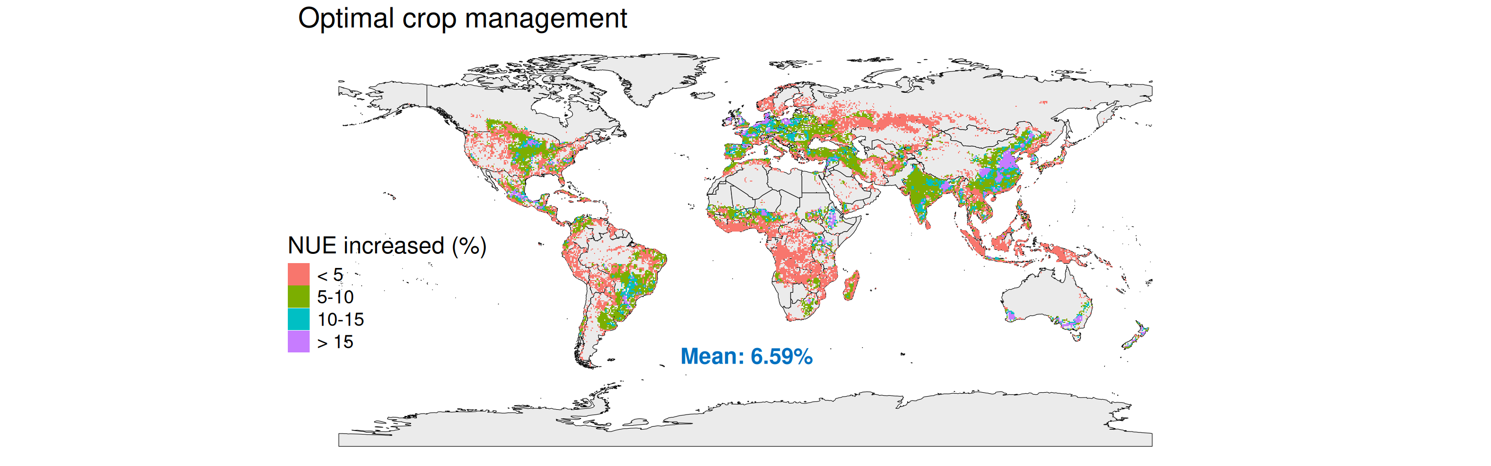
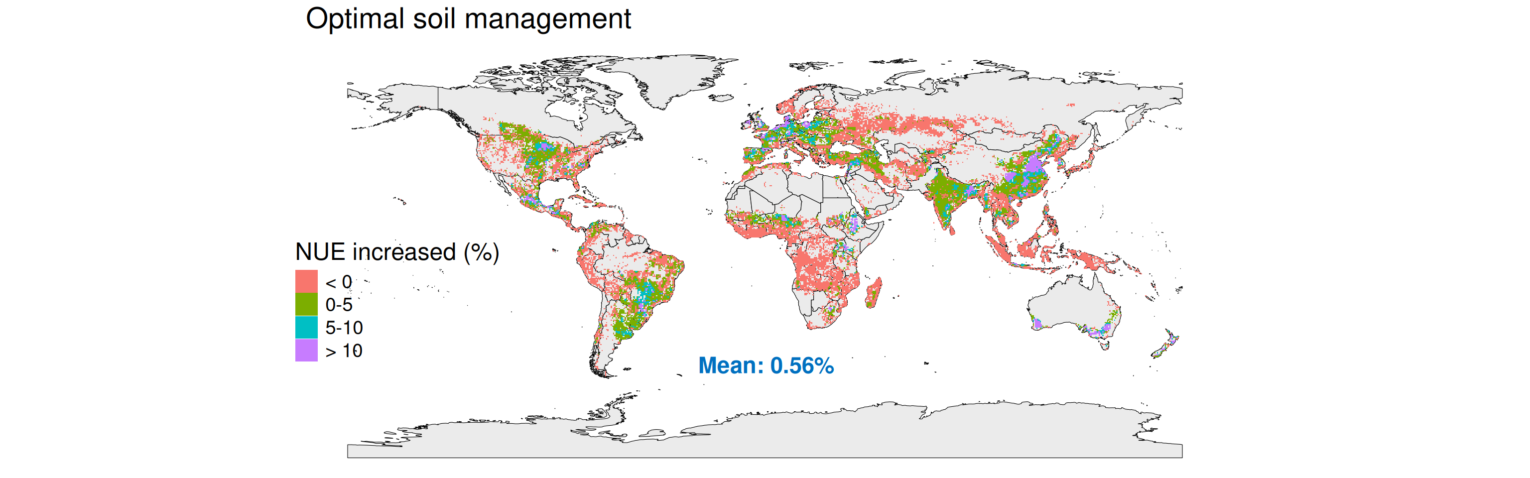
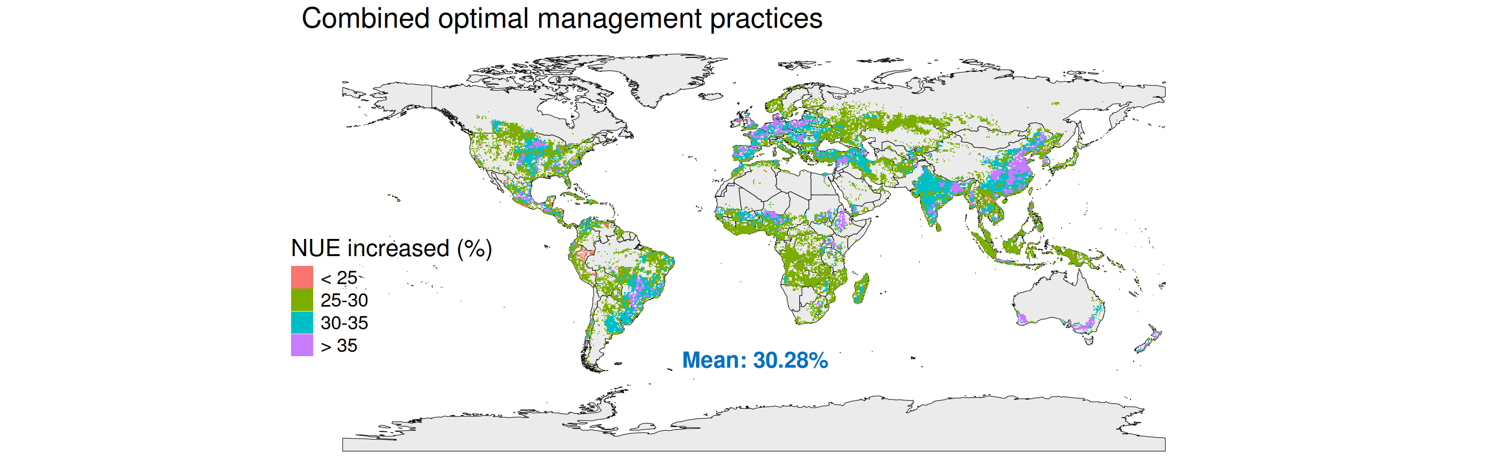
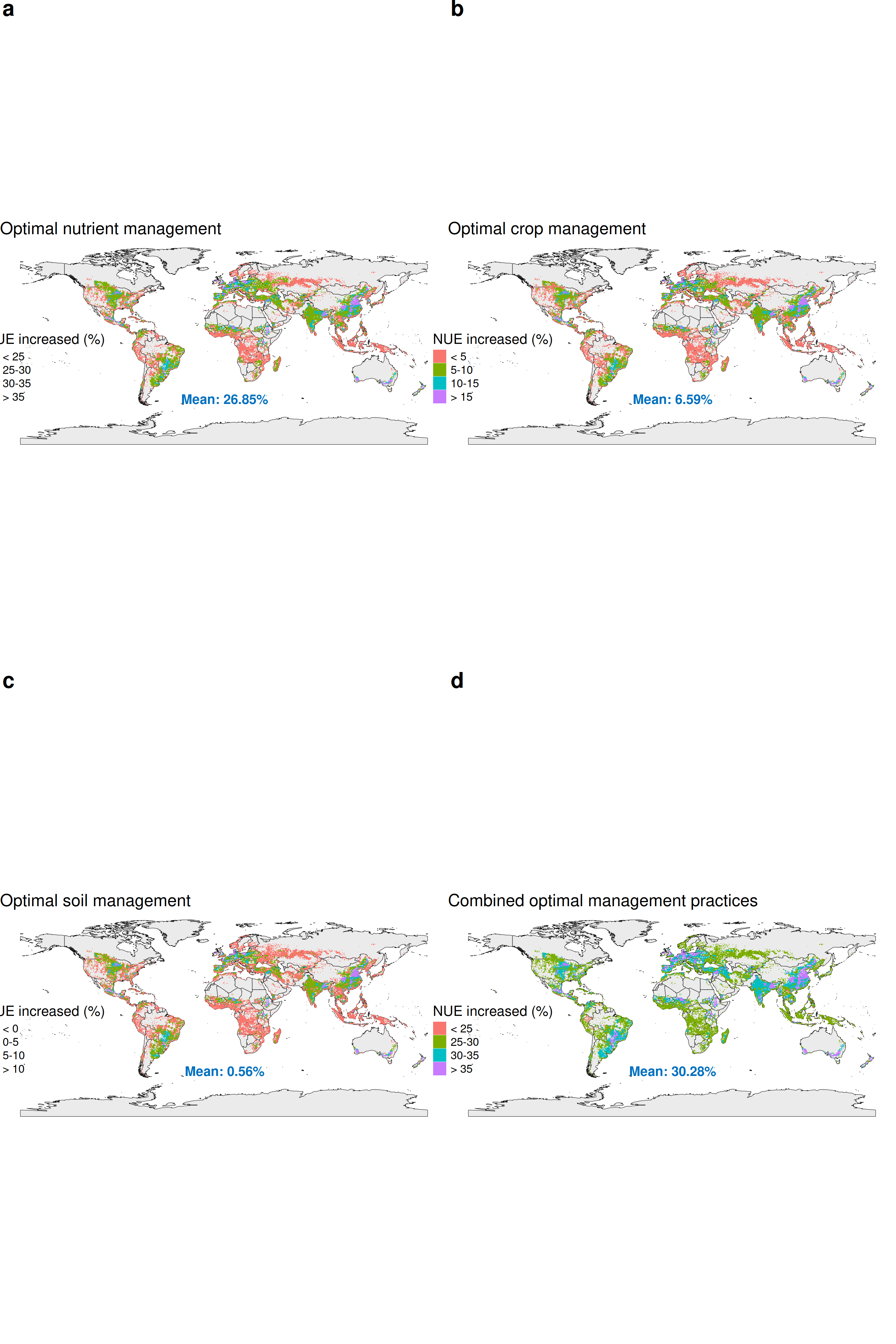
# see model structure that need to be filled in to predict NUE as function of the system properties p1 <-predict(m1,addx=T)# this is the order of input variables needed for model predictions (=newmods in predict function) m1.cols <-colnames(p1$X)# make prediction dataset for situation that soil is fertilized by both organic and inorganic fertilizers, conventional fertilizer strategy dt.new <-copy(r.dt.melt)# add the columns required for the ma model, baseline scenario # baseline is here defined as "strategy conventional", and mineral fertilizers, no biochar, no crop residue, no cover crops dt.new[, fertilizer_typeenhanced :=0] dt.new[, fertilizer_typemineral :=1] dt.new[, fertilizer_typeorganic :=0] dt.new[, fertilizer_typecombined :=0] dt.new[, rfpyes :=0] dt.new[, rftyes :=0] dt.new[, rfryes :=0] dt.new[, crop_residueyes :=0] dt.new[, cover_crop_and_crop_rotationyes :=0] dt.new[, cover_crop_and_crop_rotationyes :=fifelse(cropintensity>1,1,0)] dt.new[, `tillageno-till`:=fifelse(till_name =='no-till',1,0)]#dt.new[,`tillageno-till` := 0] dt.new[, ctryes :=fifelse(cropname=='rice',1,0)] dt.new[, ctwyes :=fifelse(cropname=='wheat',1,0)] dt.new[, ctmyes :=fifelse(cropname=='maize',1,0)] dt.new[, ph_scaled := (phw *0.1-mean(d02$ph)) /sd(d02$ph)] dt.new[, clay_scaled := (clay *0.1-mean(d02$clay)) /sd(d02$clay)] dt.new[, soc_scaled := (soc *0.1-mean(d02$soc)) /sd(d02$soc)] dt.new[, n_dose_scaled :=scale(nh4+no3+nam)] dt.new[, ndose2 :=scale((nh4+no3+nam)^2)] dt.new[, map_scaled := (pre -mean(d02$map)) /sd(d02$map)] dt.new[, mat_scaled := (mat -mean(d02$mat)) /sd(d02$mat)] dt.new[, `n_dose_scaled:soc_scaled`:= n_dose_scaled*soc_scaled] dt.new[, `rfpyes:ctmyes`:= rfpyes*ctmyes] dt.new[, `mat_scaled:ctmyes`:= mat_scaled*ctmyes]# convert to matrix, needed for rma models dt.newmod <-as.matrix(dt.new[,mget(c(m1.cols))])# predict the NUE via MD model dt.pred <-as.data.table(predict(m1,newmods = dt.newmod,addx=F))# add predictions to the data.table cols <-c('pMDmean','pMDse','pMDcil','pMDciu','pMDpil','pMDpiu') dt.new[,c(cols) := dt.pred]############################################## scenario SI0 (EE) ################################################################# make local copy dt.s10 <-copy(dt.new)# baseline mean and sd for total N input dt.fert.bs <- dt.new[,list(mean =mean(nh4+no3+nam), sd =sd(nh4+no3+nam))]# update actions taken for scenario 1 dt.s10[, fertilizer_typeenhanced :=1] dt.s10[, fertilizer_typemineral :=0] dt.s10[, fertilizer_typeorganic :=0] dt.s10[, fertilizer_typecombined :=0] dt.s10[, rfpyes :=0] dt.s10[, rftyes :=0] dt.s10[, rfryes :=0] dt.s10[, crop_residueyes :=0] dt.s10[, cover_crop_and_crop_rotationyes :=0] dt.s10[, tillageno_till :=0] dt.s10[, n_dose_scaled := ((nh4+no3+nam) *0.7- dt.fert.bs$mean)/ dt.fert.bs$sd ] dt.s10[, `n_dose_scaled:soc_scaled`:= (n_dose_scaled -0.1)*soc_scaled] dt.s10[, `rfpyes:ctmyes`:= rfpyes*ctmyes] dt.s10[, `mat_scaled:ctmyes`:= mat_scaled*ctmyes]# convert to matrix, needed for rma models dt.newmod <-as.matrix(dt.s10[,mget(c(m1.cols))])# predict the NUE via MD model dt.pred.s10 <-as.data.table(predict(m1,newmods = dt.newmod,addx=F)) dt.s10[,c(cols) := dt.pred.s10]# compare baseline with scenario # select relevant columns of the baseline dt.fin <- dt.new[,.(x,y,base = pMDmean,cropname,area)]# select relevant columns of scenario 1 and merge dt.fin <-merge(dt.fin,dt.s10[,.(x,y,s10 = pMDmean,cropname)],by=c('x','y','cropname'))# estimate relative improvement via senario 1 dt.fin[, improvement := s10 - base]# estimate area weighted mean relative improvement dt.fin <- dt.fin[,list(improvement =weighted.mean(improvement,w = area)),by =c('x','y')]# make spatial raster of the estimated improvement # convert to spatial raster r.fin <- terra::rast(dt.fin,type='xyz') terra::crs(r.fin) <-'epsg:4326'# write as output terra::writeRaster(r.fin,'tif/scenario_SI0.tif', overwrite =TRUE)############################################## scenario SI1 (CF) ################################################################# scenario SI1. the combination of measures with change in Combined fertilizer (CF vs. MF)# make local copy dt.s11 <-copy(dt.new)# baseline mean and sd for total N input dt.fert.bs <- dt.new[,list(mean =mean(nh4+no3+nam), sd =sd(nh4+no3+nam))]# update actions taken for scenario 1 dt.s11[, fertilizer_typeenhanced :=0] dt.s11[, fertilizer_typemineral :=0] dt.s11[, fertilizer_typeorganic :=0] dt.s11[, fertilizer_typecombined :=1] dt.s11[, rfpyes :=0] dt.s11[, rftyes :=0] dt.s11[, rfryes :=0] dt.s11[, crop_residueyes :=0] dt.s11[, cover_crop_and_crop_rotationyes :=0] dt.s11[, tillageno_till :=0] dt.s11[, n_dose_scaled := ((nh4+no3+nam) *0.7- dt.fert.bs$mean)/ dt.fert.bs$sd ] dt.s11[, `n_dose_scaled:soc_scaled`:= (n_dose_scaled -0.1 )*soc_scaled] dt.s11[, `rfpyes:ctmyes`:= rfpyes*ctmyes] dt.s11[, `mat_scaled:ctmyes`:= mat_scaled*ctmyes]# convert to matrix, needed for rma models dt.newmod <-as.matrix(dt.s11[,mget(c(m1.cols))])# predict the NUE via MD model dt.pred.s11 <-as.data.table(predict(m1,newmods = dt.newmod,addx=F)) dt.s11[,c(cols) := dt.pred.s11]# compare baseline with scenario # select relevant columns of the baseline dt.fin <- dt.new[,.(x,y,base = pMDmean,cropname,area)]# select relevant columns of scenario 1 and merge dt.fin <-merge(dt.fin,dt.s11[,.(x,y,s11 = pMDmean,cropname)],by=c('x','y','cropname'))# estimate relative improvement via senario 1 dt.fin[, improvement := s11 - base]# estimate area weighted mean relative improvement dt.fin <- dt.fin[,list(improvement =weighted.mean(improvement,w = area)),by =c('x','y')]# make spatial raster of the estimated improvement# convert to spatial raster r.fin <- terra::rast(dt.fin,type='xyz') terra::crs(r.fin) <-'epsg:4326'# write as output terra::writeRaster(r.fin,'tif/scenario_SI1.tif', overwrite =TRUE)############################################## scenario SI2 (OF) ################################################################# scenario SI2. the combination of measures with change in OF (OF vs. MF)# make local copy dt.s12 <-copy(dt.new)# baseline mean and sd for total N input dt.fert.bs <- dt.new[,list(mean =mean(nh4+no3+nam), sd =sd(nh4+no3+nam))]# update actions taken for scenario 1 dt.s12[, fertilizer_typeenhanced :=0] dt.s12[, fertilizer_typemineral :=0] dt.s12[, fertilizer_typeorganic :=1] dt.s12[, fertilizer_typecombined :=0] dt.s12[, rfpyes :=0] dt.s12[, rftyes :=0] dt.s12[, rfryes :=0] dt.s12[, crop_residueyes :=0] dt.s12[, cover_crop_and_crop_rotationyes :=0] dt.s12[, tillageno_till :=0] dt.s12[, n_dose_scaled := ((nh4+no3+nam) *0.7- dt.fert.bs$mean)/ dt.fert.bs$sd ] dt.s12[, `n_dose_scaled:soc_scaled`:= (n_dose_scaled -0.1 )*soc_scaled] dt.s12[, `rfpyes:ctmyes`:= rfpyes*ctmyes] dt.s12[, `mat_scaled:ctmyes`:= mat_scaled*ctmyes]# convert to matrix, needed for rma models dt.newmod <-as.matrix(dt.s12[,mget(c(m1.cols))])# predict the NUE via MD model dt.pred.s12 <-as.data.table(predict(m1,newmods = dt.newmod,addx=F)) dt.s12[,c(cols) := dt.pred.s12]# compare baseline with scenario # select relevant columns of the baseline dt.fin <- dt.new[,.(x,y,base = pMDmean,cropname,area)]# select relevant columns of scenario 1 and merge dt.fin <-merge(dt.fin,dt.s12[,.(x,y,s12 = pMDmean,cropname)],by=c('x','y','cropname'))# estimate relative improvement via senario 1 dt.fin[, improvement := s12 - base]# estimate area weighted mean relative improvement dt.fin <- dt.fin[,list(improvement =weighted.mean(improvement,w = area)),by =c('x','y')]# make spatial raster of the estimated improvement # convert to spatial raster r.fin <- terra::rast(dt.fin,type='xyz') terra::crs(r.fin) <-'epsg:4326'# write as output terra::writeRaster(r.fin,'tif/scenario_SI2.tif', overwrite =TRUE)############################################## scenario SI3 (RFP) ################################################################# scenario SI3. the combination of measures with change in RFP. (Optimized fertilizer strategy vs.Conventional fertilizer strategies)# make local copy dt.s13 <-copy(dt.new)# baseline mean and sd for total N input dt.fert.bs <- dt.new[,list(mean =mean(nh4+no3+nam), sd =sd(nh4+no3+nam))]# update actions taken for scenario 1 dt.s13[, fertilizer_typeenhanced :=0] dt.s13[, fertilizer_typemineral :=1] dt.s13[, fertilizer_typeorganic :=0] dt.s13[, fertilizer_typecombined :=0] dt.s13[, rfpyes :=1] dt.s13[, rftyes :=0] dt.s13[, rfryes :=0] dt.s13[, crop_residueyes :=0] dt.s13[, cover_crop_and_crop_rotationyes :=0] dt.s13[, tillageno_till :=0] dt.s13[, n_dose_scaled := ((nh4+no3+nam) *0.7- dt.fert.bs$mean)/ dt.fert.bs$sd ] dt.s13[, `n_dose_scaled:soc_scaled`:= (n_dose_scaled -0.1 )*soc_scaled] dt.s13[, `rfpyes:ctmyes`:= rfpyes*ctmyes] dt.s13[, `mat_scaled:ctmyes`:= mat_scaled*ctmyes]# convert to matrix, needed for rma models dt.newmod <-as.matrix(dt.s13[,mget(c(m1.cols))])# predict the NUE via MD model dt.pred.s13 <-as.data.table(predict(m1,newmods = dt.newmod,addx=F)) dt.s13[,c(cols) := dt.pred.s13]# compare baseline with scenario # select relevant columns of the baseline dt.fin <- dt.new[,.(x,y,base = pMDmean,cropname,area)]# select relevant columns of scenario 1 and merge dt.fin <-merge(dt.fin,dt.s13[,.(x,y,s13 = pMDmean,cropname)],by=c('x','y','cropname'))# estimate relative improvement via senario 1 dt.fin[, improvement := s13 - base]# estimate area weighted mean relative improvement dt.fin <- dt.fin[,list(improvement =weighted.mean(improvement,w = area)),by =c('x','y')]# make spatial raster of the estimated improvement # convert to spatial raster r.fin <- terra::rast(dt.fin,type='xyz') terra::crs(r.fin) <-'epsg:4326'# write as output terra::writeRaster(r.fin,'tif/scenario_SI3.tif', overwrite =TRUE)############################################## scenario SI4 (RFR) ################################################################# scenario SI4. the combination of measures with change in RFR. (Optimized fertilizer strategy vs.Conventional fertilizer strategies)# make local copy dt.s14 <-copy(dt.new)# baseline mean and sd for total N input dt.fert.bs <- dt.new[,list(mean =mean(nh4+no3+nam), sd =sd(nh4+no3+nam))]# update actions taken for scenario 1 dt.s14[, fertilizer_typeenhanced :=0] dt.s14[, fertilizer_typemineral :=1] dt.s14[, fertilizer_typeorganic :=0] dt.s14[, fertilizer_typecombined :=0] dt.s14[, rfpyes :=0] dt.s14[, rftyes :=0] dt.s14[, rfryes :=1] dt.s14[, crop_residueyes :=0] dt.s14[, cover_crop_and_crop_rotationyes :=0] dt.s14[, tillageno_till :=0] dt.s14[, n_dose_scaled := ((nh4+no3+nam) *0.7- dt.fert.bs$mean)/ dt.fert.bs$sd ] dt.s14[, `n_dose_scaled:soc_scaled`:= (n_dose_scaled -0.1 )*soc_scaled] dt.s14[, `rfpyes:ctmyes`:= rfpyes*ctmyes] dt.s14[, `mat_scaled:ctmyes`:= mat_scaled*ctmyes]# convert to matrix, needed for rma models dt.newmod <-as.matrix(dt.s14[,mget(c(m1.cols))])# predict the NUE via MD model dt.pred.s14 <-as.data.table(predict(m1,newmods = dt.newmod,addx=F)) dt.s14[,c(cols) := dt.pred.s14]# compare baseline with scenario # select relevant columns of the baseline dt.fin <- dt.new[,.(x,y,base = pMDmean,cropname,area)]# select relevant columns of scenario 1 and merge dt.fin <-merge(dt.fin,dt.s14[,.(x,y,s14 = pMDmean,cropname)],by=c('x','y','cropname'))# estimate relative improvement via senario 1 dt.fin[, improvement := s14 - base]# estimate area weighted mean relative improvement dt.fin <- dt.fin[,list(improvement =weighted.mean(improvement,w = area)),by =c('x','y')]# make spatial raster of the estimated improvement # convert to spatial raster r.fin <- terra::rast(dt.fin,type='xyz') terra::crs(r.fin) <-'epsg:4326'# write as output terra::writeRaster(r.fin,'tif/scenario_SI4.tif', overwrite =TRUE)############################################## scenario SI5 (RFT) ################################################################# scenario SI5. the combination of measures with change in RFT. (Optimized fertilizer strategy vs.Conventional fertilizer strategies)# make local copy dt.s15 <-copy(dt.new)# baseline mean and sd for total N input dt.fert.bs <- dt.new[,list(mean =mean(nh4+no3+nam), sd =sd(nh4+no3+nam))]# update actions taken for scenario 1 dt.s15[, fertilizer_typeenhanced :=0] dt.s15[, fertilizer_typemineral :=1] dt.s15[, fertilizer_typeorganic :=0] dt.s15[, fertilizer_typecombined :=0] dt.s15[, rfpyes :=0] dt.s15[, rftyes :=1] dt.s15[, rfryes :=0] dt.s15[, crop_residueyes :=0] dt.s15[, cover_crop_and_crop_rotationyes :=0] dt.s15[, tillageno_till :=0] dt.s15[, n_dose_scaled := ((nh4+no3+nam) *0.7- dt.fert.bs$mean)/ dt.fert.bs$sd ] dt.s15[, `n_dose_scaled:soc_scaled`:= (n_dose_scaled -0.1 )*soc_scaled] dt.s15[, `rfpyes:ctmyes`:= rfpyes*ctmyes] dt.s15[, `mat_scaled:ctmyes`:= mat_scaled*ctmyes]# convert to matrix, needed for rma models dt.newmod <-as.matrix(dt.s15[,mget(c(m1.cols))])# predict the NUE via MD model dt.pred.s15 <-as.data.table(predict(m1,newmods = dt.newmod,addx=F)) dt.s15[,c(cols) := dt.pred.s15]# compare baseline with scenario # select relevant columns of the baseline dt.fin <- dt.new[,.(x,y,base = pMDmean,cropname,area)]# select relevant columns of scenario 1 and merge dt.fin <-merge(dt.fin,dt.s15[,.(x,y,s15 = pMDmean,cropname)],by=c('x','y','cropname'))# estimate relative improvement via senario 1 dt.fin[, improvement := s15 - base]# estimate area weighted mean relative improvement dt.fin <- dt.fin[,list(improvement =weighted.mean(improvement,w = area)),by =c('x','y')]# make spatial raster of the estimated improvement # convert to spatial raster r.fin <- terra::rast(dt.fin,type='xyz') terra::crs(r.fin) <-'epsg:4326'# write as output terra::writeRaster(r.fin,'tif/scenario_SI5.tif', overwrite =TRUE)############################################## scenario SI7 (RES) ################################################################# scenario SI7. the combination of measures with change in RES. (Optimized fertilizer strategy vs.Conventional fertilizer strategies)# make local copy dt.s17 <-copy(dt.new)# baseline mean and sd for total N input dt.fert.bs <- dt.new[,list(mean =mean(nh4+no3+nam), sd =sd(nh4+no3+nam))]# update actions taken for scenario 1 dt.s17[, fertilizer_typeenhanced :=0] dt.s17[, fertilizer_typemineral :=1] dt.s17[, fertilizer_typeorganic :=0] dt.s17[, fertilizer_typecombined :=0] dt.s17[, rfpyes :=0] dt.s17[, rftyes :=0] dt.s17[, rfryes :=0] dt.s17[, crop_residueyes :=1] dt.s17[, cover_crop_and_crop_rotationyes :=0] dt.s17[, tillageno_till :=0] dt.s17[, n_dose_scaled := ((nh4+no3+nam) *0.7- dt.fert.bs$mean)/ dt.fert.bs$sd ] dt.s17[, `n_dose_scaled:soc_scaled`:= (n_dose_scaled -0.1 )*soc_scaled] dt.s17[, `rfpyes:ctmyes`:= rfpyes*ctmyes] dt.s17[, `mat_scaled:ctmyes`:= mat_scaled*ctmyes]# convert to matrix, needed for rma models dt.newmod <-as.matrix(dt.s17[,mget(c(m1.cols))])# predict the NUE via MD model dt.pred.s17 <-as.data.table(predict(m1,newmods = dt.newmod,addx=F)) dt.s17[,c(cols) := dt.pred.s17]# compare baseline with scenario # select relevant columns of the baseline dt.fin <- dt.new[,.(x,y,base = pMDmean,cropname,area)]# select relevant columns of scenario 1 and merge dt.fin <-merge(dt.fin,dt.s17[,.(x,y,s17 = pMDmean,cropname)],by=c('x','y','cropname'))# estimate relative improvement via senario 1 dt.fin[, improvement := s17 - base]# estimate area weighted mean relative improvement dt.fin <- dt.fin[,list(improvement =weighted.mean(improvement,w = area)),by =c('x','y')]# make spatial raster of the estimated improvement # convert to spatial raster r.fin <- terra::rast(dt.fin,type='xyz') terra::crs(r.fin) <-'epsg:4326'# write as output terra::writeRaster(r.fin,'tif/scenario_SI7.tif', overwrite =TRUE)############################################## scenario SI8 (CC/ROT) ################################################################# scenario SI8. the combination of measures with change in CC/ROT. (Optimized fertilizer strategy vs.Conventional fertilizer strategies)# make local copy dt.s18 <-copy(dt.new)# baseline mean and sd for total N input dt.fert.bs <- dt.new[,list(mean =mean(nh4+no3+nam), sd =sd(nh4+no3+nam))]# update actions taken for scenario 1 dt.s18[, fertilizer_typeenhanced :=0] dt.s18[, fertilizer_typemineral :=1] dt.s18[, fertilizer_typeorganic :=0] dt.s18[, fertilizer_typecombined :=0] dt.s18[, rfpyes :=0] dt.s18[, rftyes :=0] dt.s18[, rfryes :=0] dt.s18[, crop_residueyes :=0] dt.s18[, cover_crop_and_crop_rotationyes :=1] dt.s18[, tillageno_till :=0] dt.s18[, n_dose_scaled := ((nh4+no3+nam) *0.7- dt.fert.bs$mean)/ dt.fert.bs$sd ] dt.s18[, `n_dose_scaled:soc_scaled`:= (n_dose_scaled -0.1 )*soc_scaled] dt.s18[, `rfpyes:ctmyes`:= rfpyes*ctmyes] dt.s18[, `mat_scaled:ctmyes`:= mat_scaled*ctmyes]# convert to matrix, needed for rma models dt.newmod <-as.matrix(dt.s18[,mget(c(m1.cols))])# predict the NUE via MD model dt.pred.s18 <-as.data.table(predict(m1,newmods = dt.newmod,addx=F)) dt.s18[,c(cols) := dt.pred.s18]# compare baseline with scenario # select relevant columns of the baseline dt.fin <- dt.new[,.(x,y,base = pMDmean,cropname,area)]# select relevant columns of scenario 1 and merge dt.fin <-merge(dt.fin,dt.s18[,.(x,y,s18 = pMDmean,cropname)],by=c('x','y','cropname'))# estimate relative improvement via senario 1 dt.fin[, improvement := s18 - base]# estimate area weighted mean relative improvement dt.fin <- dt.fin[,list(improvement =weighted.mean(improvement,w = area)),by =c('x','y')]# make spatial raster of the estimated improvement # convert to spatial raster r.fin <- terra::rast(dt.fin,type='xyz') terra::crs(r.fin) <-'epsg:4326'# write as output terra::writeRaster(r.fin,'tif/scenario_SI8.tif', overwrite =TRUE)#################################################################################################################################################### ############################################## scenario 1 (Nutrient management) ################################################################# scenario 1. the combination of measures with change in RFR, RFT and BC. (Optimized fertilizer strategy vs.Conventional fertilizer strategies)# make local copy dt.s1 <-copy(dt.new)# baseline mean and sd for total N input dt.fert.bs <- dt.new[,list(mean =mean(nh4+no3+nam), sd =sd(nh4+no3+nam))]# update actions taken for scenario 1 dt.s1[, fertilizer_typeenhanced :=1] dt.s1[, fertilizer_typemineral :=0] dt.s1[, fertilizer_typeorganic :=1] dt.s1[, fertilizer_typecombined :=1] dt.s1[, rfpyes :=1] dt.s1[, rftyes :=1] dt.s1[, rfryes :=1] dt.s1[, crop_residueyes :=0] dt.s1[, cover_crop_and_crop_rotationyes :=0] dt.s1[, tillageno_till :=0] dt.s1[, n_dose_scaled := ((nh4+no3+nam) *0.7- dt.fert.bs$mean)/ dt.fert.bs$sd ] dt.s1[, `n_dose_scaled:soc_scaled`:= (n_dose_scaled -0.1 )*soc_scaled] dt.s1[, `rfpyes:ctmyes`:= rfpyes*ctmyes] dt.s1[, `mat_scaled:ctmyes`:= mat_scaled*ctmyes]# convert to matrix, needed for rma models dt.newmod <-as.matrix(dt.s1[,mget(c(m1.cols))])# predict the NUE via MD model dt.pred.s1 <-as.data.table(predict(m1,newmods = dt.newmod,addx=F)) dt.s1[,c(cols) := dt.pred.s1]# compare baseline with scenario # select relevant columns of the baseline dt.fin <- dt.new[,.(x,y,base = pMDmean,cropname,area)]# select relevant columns of scenario 1 and merge dt.fin <-merge(dt.fin,dt.s1[,.(x,y,s1 = pMDmean,cropname)],by=c('x','y','cropname'))# estimate relative improvement via senario 1 dt.fin[, improvement := s1 - base]# estimate area weighted mean relative improvement dt.fin <- dt.fin[,list(improvement =weighted.mean(improvement,w = area)),by =c('x','y')]# make spatial raster of the estimated improvement # convert to spatial raster r.fin <- terra::rast(dt.fin,type='xyz') terra::crs(r.fin) <-'epsg:4326'# write as output terra::writeRaster(r.fin,'tif/scenario_1.tif', overwrite =TRUE)############################################## scenario 2 (crop management)################################################################# scenario 2. the combination of measures with change in RES, CC, ROT (Optimized crop management vs. Conventional crop management)# make local copy dt.s2 <-copy(dt.new)# baseline mean and sd for total N input dt.fert.bs <- dt.new[,list(mean =mean(nh4+no3+nam), sd =sd(nh4+no3+nam))]# update actions taken for scenario 3 dt.s2[, fertilizer_typeenhanced :=0] dt.s2[, fertilizer_typemineral :=1] dt.s2[, fertilizer_typeorganic :=0] dt.s2[, fertilizer_typecombined :=0] dt.s2[, rfpyes :=0] dt.s2[, rftyes :=0] dt.s2[, rfryes :=0] dt.s2[, crop_residueyes :=1] dt.s2[, cover_crop_and_crop_rotationyes :=1] dt.s2[, tillageno_till :=0] dt.s2[, n_dose_scaled := ((nh4+no3+nam) *0.7- dt.fert.bs$mean)/ dt.fert.bs$sd ] dt.s2[, `n_dose_scaled:soc_scaled`:= (n_dose_scaled -0.1 )*soc_scaled] dt.s2[, `rfpyes:ctmyes`:= rfpyes*ctmyes] dt.s2[, `mat_scaled:ctmyes`:= mat_scaled*ctmyes]# convert to matrix, needed for rma models dt.newmod <-as.matrix(dt.s2[,mget(c(m1.cols))])# predict the NUE via MD model dt.pred.s2 <-as.data.table(predict(m1,newmods = dt.newmod,addx=F)) dt.s2[,c(cols) := dt.pred.s2]# compare baseline with scenario # select relevant columns of the baseline dt.fin <- dt.new[,.(x,y,base = pMDmean,cropname,area)]# select relevant columns of scenario 1 and merge dt.fin <-merge(dt.fin,dt.s2[,.(x,y,s2 = pMDmean,cropname)],by=c('x','y','cropname'))# estimate relative improvement via senario 1 dt.fin[, improvement := s2 - base]# estimate area weighted mean relative improvement dt.fin <- dt.fin[,list(improvement =weighted.mean(improvement,w = area)),by =c('x','y')]# make spatial raster of the estimated improvement # convert to spatial raster r.fin <- terra::rast(dt.fin,type='xyz') terra::crs(r.fin) <-'epsg:4326'# write as output terra::writeRaster(r.fin,'tif/scenario_2.tif', overwrite =TRUE)############################################## scenario 3 (NT/RT) ################################################################# scenario 3. the combination of measures with change in NT/RT. (Optimized fertilizer strategy vs.Conventional fertilizer strategies)# make local copy dt.s3 <-copy(dt.new)# baseline mean and sd for total N input dt.fert.bs <- dt.new[,list(mean =mean(nh4+no3+nam), sd =sd(nh4+no3+nam))]# update actions taken for scenario 1 dt.s3[, fertilizer_typeenhanced :=0] dt.s3[, fertilizer_typemineral :=1] dt.s3[, fertilizer_typeorganic :=0] dt.s3[, fertilizer_typecombined :=0] dt.s3[, rfpyes :=0] dt.s3[, rftyes :=0] dt.s3[, rfryes :=0] dt.s3[, crop_residueyes :=0] dt.s3[, cover_crop_and_crop_rotationyes :=0] dt.s3[, `tillageno-till`:=1] dt.s3[, n_dose_scaled := ((nh4+no3+nam) *0.7- dt.fert.bs$mean)/ dt.fert.bs$sd ] dt.s3[, `n_dose_scaled:soc_scaled`:= (n_dose_scaled -0.1 )*soc_scaled] dt.s3[, `rfpyes:ctmyes`:= rfpyes*ctmyes] dt.s3[, `mat_scaled:ctmyes`:= mat_scaled*ctmyes]# convert to matrix, needed for rma models dt.newmod <-as.matrix(dt.s3[,mget(c(m1.cols))])# predict the NUE via MD model dt.pred.s3 <-as.data.table(predict(m1,newmods = dt.newmod,addx=F)) dt.s3[,c(cols) := dt.pred.s3]# compare baseline with scenario # select relevant columns of the baseline dt.fin <- dt.new[,.(x,y,base = pMDmean,cropname,area)]# select relevant columns of scenario 1 and merge dt.fin <-merge(dt.fin,dt.s3[,.(x,y,s3 = pMDmean,cropname)],by=c('x','y','cropname'))# estimate relative improvement via senario 1 dt.fin[, improvement := s3 - base]# estimate area weighted mean relative improvement dt.fin <- dt.fin[,list(improvement =weighted.mean(improvement,w = area)),by =c('x','y')]# make spatial raster of the estimated improvement # convert to spatial raster r.fin <- terra::rast(dt.fin,type='xyz') terra::crs(r.fin) <-'epsg:4326'# write as output terra::writeRaster(r.fin,'tif/scenario_3.tif', overwrite =TRUE)############################################## scenario 4 (combination)################################################################# scenario 4. the combination of measures with change in EE, CF, RFR, RFT, BC, RES, CC, ROT# make local copy dt.s4 <-copy(dt.new)# baseline mean and sd for total N input dt.fert.bs <- dt.new[,list(mean =mean(nh4+no3+nam), sd =sd(nh4+no3+nam))]# update actions taken for scenario 3 dt.s4[, fertilizer_typeenhanced :=1] dt.s4[, fertilizer_typemineral :=0] dt.s4[, fertilizer_typeorganic :=1] dt.s4[, fertilizer_typecombined :=1] dt.s4[, rfpyes :=1] dt.s4[, rftyes :=1] dt.s4[, rfryes :=1] dt.s4[, crop_residueyes :=1] dt.s4[, cover_crop_and_crop_rotationyes :=1] dt.s4[, tillageno_till :=1] dt.s4[, n_dose_scaled := ((nh4+no3+nam) *0.7- dt.fert.bs$mean)/ dt.fert.bs$sd ] dt.s4[, `n_dose_scaled:soc_scaled`:= (n_dose_scaled -0.1 )*soc_scaled] dt.s4[, `rfpyes:ctmyes`:= rfpyes*ctmyes] dt.s4[, `mat_scaled:ctmyes`:= mat_scaled*ctmyes]# convert to matrix, needed for rma models dt.newmod <-as.matrix(dt.s4[,mget(c(m1.cols))])# predict the NUE via MD model dt.pred.s4 <-as.data.table(predict(m1,newmods = dt.newmod,addx=F)) dt.s4[,c(cols) := dt.pred.s4]# compare baseline with scenario # select relevant columns of the baseline dt.fin <- dt.new[,.(x,y,base = pMDmean,cropname,area)]# select relevant columns of scenario 1 and merge dt.fin <-merge(dt.fin,dt.s4[,.(x,y,s4 = pMDmean,cropname)],by=c('x','y','cropname'))# estimate relative improvement via senario 1 dt.fin[, improvement := s4 - base]# estimate area weighted mean relative improvement dt.fin <- dt.fin[,list(improvement =weighted.mean(improvement,w = area)),by =c('x','y')]# make spatial raster of the estimated improvement # convert to spatial raster r.fin <- terra::rast(dt.fin,type='xyz') terra::crs(r.fin) <-'epsg:4326'# write as output terra::writeRaster(r.fin,'tif/scenario_4.tif', overwrite =TRUE) ################################################################################################################################ plottinglibrary(ggplot2)library(sf)
Linking to GEOS 3.12.1, GDAL 3.8.4, PROJ 9.4.0; sf_use_s2() is TRUE
library(rnaturalearth)library(rnaturalearthdata)
Attaching package: 'rnaturalearthdata'
The following object is masked from 'package:rnaturalearth':

    countries110
library(terra)library(cowplot)library(vcd)
Loading required package: grid
Attaching package: 'grid'
The following object is masked from 'package:terra':

    depth
Attaching package: 'vcd'
The following objects are masked from 'package:terra':

    mosaic, sieve
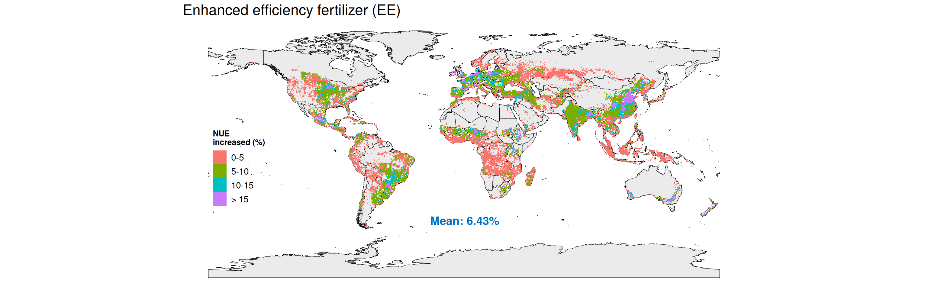
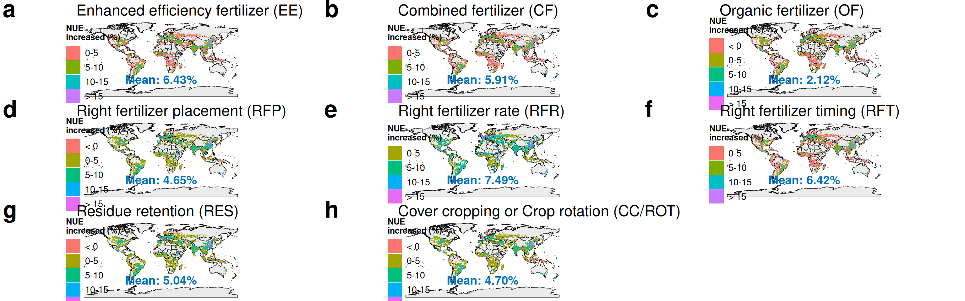
######################################### scenario_SI0 (EE) ########################################################### set themetheme_set(theme_bw())# get the raster to plot r10 <- terra::rast('tif/scenario_SI0.tif')# convert to data.frame r10.p <-as.data.frame(r10,xy=TRUE)# Exclude outliers greater than 70% r10.p <- r10.p[r10.p$improvement <70,]# get base world map world <-ne_countries(scale ="medium", returnclass ="sf")#plot a basic world map plot p10 <-ggplot(data = world) +geom_sf(color ="black", fill ="gray92") +geom_tile(data = r10.p,aes(x=x,y=y, name ='none',fill =cut(improvement,limits =c(-10,1000), breaks=c(-10,0,5,10,15,1000),labels =c('< 0','0-5','5-10','10-15','> 15')))) +# scale_fill_gradientn(colours = rainbow(3)) +#scale_fill_viridis_c()+ theme_void() +theme(legend.position =c(0.1,0.45), text =element_text(size =15),legend.background =element_rect(fill =NA,color =NA),panel.border =element_blank()) +labs(fill ='NUE\nincreased (%)') +theme(legend.title =element_text(color ="black", size =10, face ="bold"),legend.text =element_text(color ="black", size =11))+#theme(legend.position = "none")+#theme(NULL)+xlab("Longitude") +ylab("Latitude") +ggtitle("Enhanced efficiency fertilizer (EE)") +annotate("text",x=0.5,y=-50,label="Mean: 6.43%",size=5, colour="#0070C0",fontface ="bold")+# ggtitle("World map", subtitle = "Mean change for scenario 1") +coord_sf(crs =4326)
Warning in geom_tile(data = r10.p, aes(x = x, y = y, name = "none", fill =
cut(improvement, : Ignoring unknown aesthetics: name
Warning: A numeric `legend.position` argument in `theme()` was deprecated in ggplot2
3.5.0.
ℹ Please use the `legend.position.inside` argument of `theme()` instead.
p10
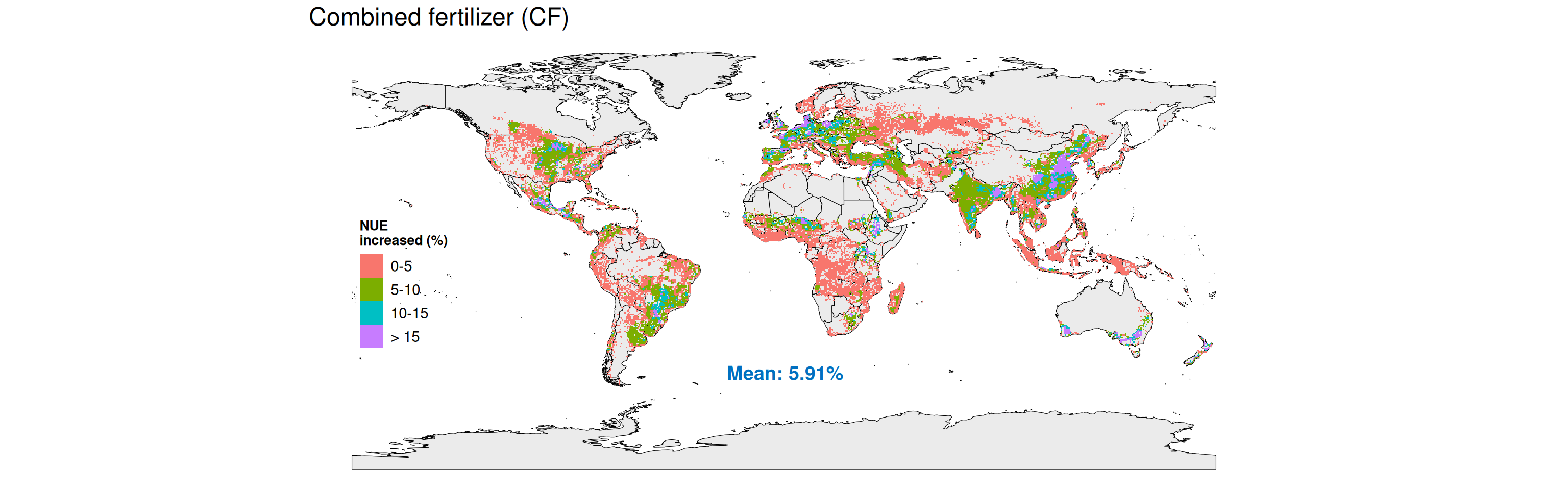
########################################### scenario_SI1 (CF) ######################################################### set themetheme_set(theme_bw())# get the raster to plot r11 <- terra::rast('tif/scenario_SI1.tif')# convert to data.frame r11.p <-as.data.frame(r11,xy=TRUE)# Exclude outliers greater than 70% r11.p <- r11.p[r11.p$improvement <70,]# get base world map world <-ne_countries(scale ="medium", returnclass ="sf")# plot a basic world map plot p11 <-ggplot(data = world) +geom_sf(color ="black", fill ="gray92") +geom_tile(data = r11.p,aes(x=x,y=y, name ='none',fill =cut(improvement,breaks=c(-10,0,5,10,15,1000),labels =c('< 0','0-5','5-10','10-15','> 15') ))) +theme_void() +theme(legend.position =c(0.1,0.45), text =element_text(size =15),legend.background =element_rect(fill =NA,color =NA),panel.border =element_blank()) +labs(fill ='NUE\nincreased (%)') +theme(legend.title =element_text(color ="black", size =10, face ="bold"),legend.text =element_text(color ="black", size =11))+#theme(legend.position = "none")+xlab("Longitude") +ylab("Latitude") +ggtitle("Combined fertilizer (CF)") +#ggtitle("World map", subtitle = "Mean change for scenario 4") +annotate("text",x=0.5,y=-50,label="Mean: 5.91%",size=5, colour="#0070C0",fontface ="bold")+coord_sf(crs =4326)
Warning in geom_tile(data = r11.p, aes(x = x, y = y, name = "none", fill =
cut(improvement, : Ignoring unknown aesthetics: name
p11
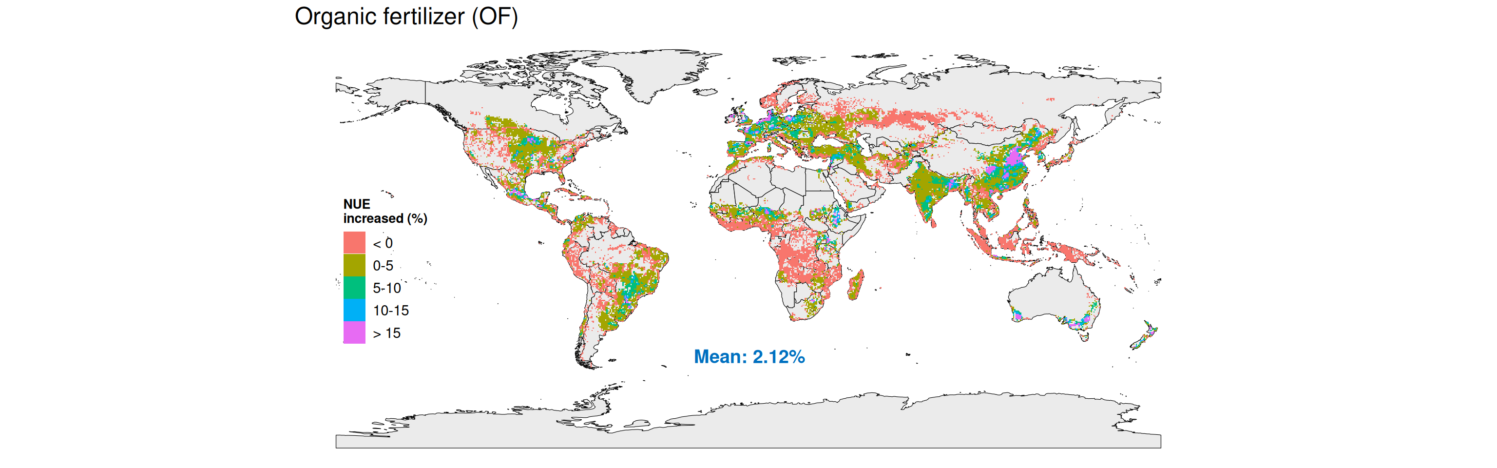
########################################### scenario_SI2 (OF) ######################################################### set themetheme_set(theme_bw())# get the raster to plot r12 <- terra::rast('tif/scenario_SI2.tif')# convert to data.frame r12.p <-as.data.frame(r12,xy=TRUE)# Exclude outliers greater than 70% r12.p <- r12.p[r12.p$improvement <70,]# get base world map world <-ne_countries(scale ="medium", returnclass ="sf")# plot a basic world map plot p12 <-ggplot(data = world) +geom_sf(color ="black", fill ="gray92") +geom_tile(data = r12.p,aes(x=x,y=y, name ='none',fill =cut(improvement,breaks=c(-10,0,5,10,15,1000),labels =c('< 0','0-5','5-10','10-15','> 15') ))) +theme_void() +theme(legend.position =c(0.1,0.45), text =element_text(size =15),legend.background =element_rect(fill =NA,color =NA),panel.border =element_blank()) +labs(fill ='NUE\nincreased (%)') +theme(legend.title =element_text(color ="black", size =10, face ="bold"),legend.text =element_text(color ="black", size =11))+#theme(legend.position = "none")+xlab("Longitude") +ylab("Latitude") +ggtitle("Organic fertilizer (OF)") +#ggtitle("World map", subtitle = "Mean change for scenario 4") +annotate("text",x=0.5,y=-50,label="Mean: 2.12%",size=5, colour="#0070C0",fontface ="bold")+coord_sf(crs =4326)
Warning in geom_tile(data = r12.p, aes(x = x, y = y, name = "none", fill =
cut(improvement, : Ignoring unknown aesthetics: name
p12
########################################### scenario_SI3 (RFP) ######################################################### set themetheme_set(theme_bw())# get the raster to plot r13 <- terra::rast('tif/scenario_SI3.tif')# convert to data.frame r13.p <-as.data.frame(r13,xy=TRUE)# Exclude outliers greater than 70% r13.p <- r13.p[r13.p$improvement <70,]# get base world map world <-ne_countries(scale ="medium", returnclass ="sf")# plot a basic world map plot p13 <-ggplot(data = world) +geom_sf(color ="black", fill ="gray92") +geom_tile(data = r13.p,aes(x=x,y=y, name ='none',fill =cut(improvement,breaks=c(-10,0,5,10,15,1000),labels =c('< 0','0-5','5-10','10-15','> 15') ))) +theme_void() +theme(legend.position =c(0.1,0.45), text =element_text(size =15),legend.background =element_rect(fill =NA,color =NA),panel.border =element_blank()) +labs(fill ='NUE\nincreased (%)') +theme(legend.title =element_text(color ="black", size =10, face ="bold"),legend.text =element_text(color ="black", size =11))+#theme(legend.position = "none")+xlab("Longitude") +ylab("Latitude") +ggtitle("Right fertilizer placement (RFP)") +#ggtitle("World map", subtitle = "Mean change for scenario 4") +annotate("text",x=0.5,y=-50,label="Mean: 4.65%",size=5, colour="#0070C0",fontface ="bold")+coord_sf(crs =4326)
Warning in geom_tile(data = r13.p, aes(x = x, y = y, name = "none", fill =
cut(improvement, : Ignoring unknown aesthetics: name
p13
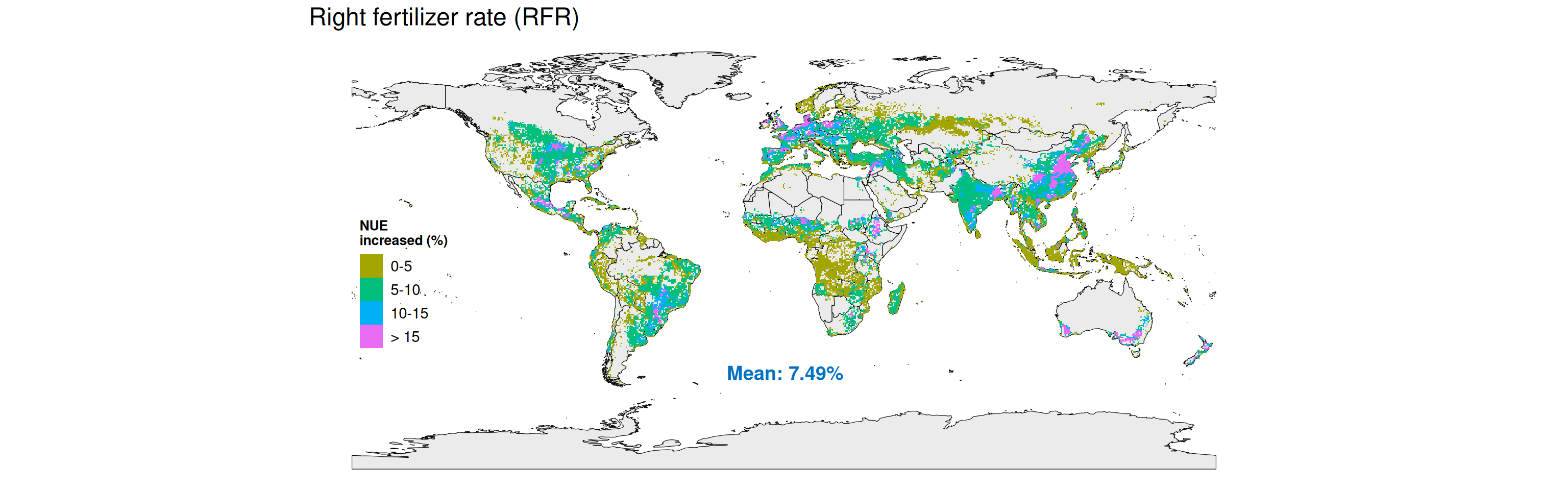
########################################### scenario_SI4 (RFR) ######################################################### set themetheme_set(theme_bw())# get the raster to plot r14 <- terra::rast('tif/scenario_SI4.tif')# convert to data.frame r14.p <-as.data.frame(r14,xy=TRUE)# Exclude outliers greater than 70% r14.p <- r14.p[r14.p$improvement <70,]# get base world map world <-ne_countries(scale ="medium", returnclass ="sf")# plot a basic world map plot p14 <-ggplot(data = world) +geom_sf(color ="black", fill ="gray92") +geom_tile(data = r14.p,aes(x=x,y=y, name ='none',fill =cut(improvement,limits =c(-10,1000), breaks=c(0,5,10,15,1000),labels =c('0-5','5-10','10-15','> 15') ))) +theme_void() +theme(legend.position =c(0.1,0.45), text =element_text(size =15),legend.background =element_rect(fill =NA,color =NA),panel.border =element_blank()) +labs(fill ='NUE\nincreased (%)') +theme(legend.title =element_text(color ="black", size =10, face ="bold"),legend.text =element_text(color ="black", size =11))+scale_fill_manual(values =c("#a3a500", "#00bf7d", "#00b0f6","#e76bf3"))+#theme(legend.position = "none")+xlab("Longitude") +ylab("Latitude") +ggtitle("Right fertilizer rate (RFR)") +#ggtitle("World map", subtitle = "Mean change for scenario 4") +annotate("text",x=0.5,y=-50,label="Mean: 7.49%",size=5, colour="#0070C0",fontface ="bold")+coord_sf(crs =4326)
Warning in geom_tile(data = r14.p, aes(x = x, y = y, name = "none", fill =
cut(improvement, : Ignoring unknown aesthetics: name
p14
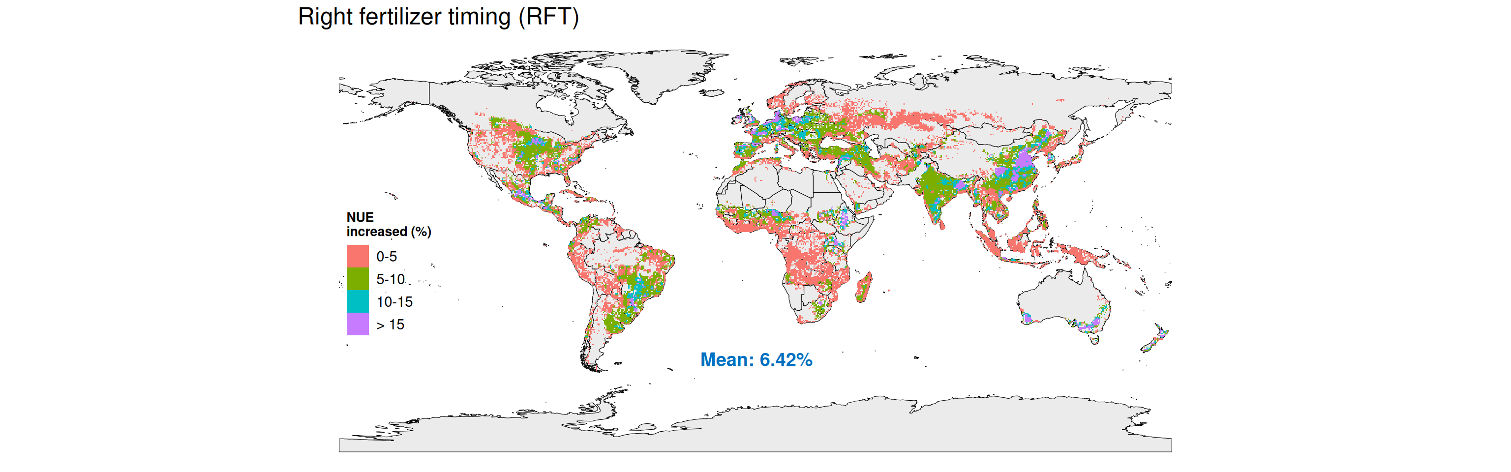
########################################### scenario_SI5 (RFT) ######################################################### set themetheme_set(theme_bw())# get the raster to plot r15 <- terra::rast('tif/scenario_SI5.tif')# convert to data.frame r15.p <-as.data.frame(r15,xy=TRUE)# Exclude outliers greater than 70% r15.p <- r15.p[r15.p$improvement <70,]# get base world map world <-ne_countries(scale ="medium", returnclass ="sf")# plot a basic world map plot p15 <-ggplot(data = world) +geom_sf(color ="black", fill ="gray92") +geom_tile(data = r15.p,aes(x=x,y=y, name ='none',fill =cut(improvement,breaks=c(-10,0,5,10,15,1000),labels =c('< 0','0-5','5-10','10-15','> 15') ))) +theme_void() +theme(legend.position =c(0.1,0.45), text =element_text(size =15),legend.background =element_rect(fill =NA,color =NA),panel.border =element_blank()) +labs(fill ='NUE\nincreased (%)') +theme(legend.title =element_text(color ="black", size =10, face ="bold"),legend.text =element_text(color ="black", size =11))+#theme(legend.position = "none")+xlab("Longitude") +ylab("Latitude") +ggtitle("Right fertilizer timing (RFT)") +#ggtitle("World map", subtitle = "Mean change for scenario 4") +annotate("text",x=0.5,y=-50,label="Mean: 6.42%",size=5, colour="#0070C0",fontface ="bold")+coord_sf(crs =4326)
Warning in geom_tile(data = r15.p, aes(x = x, y = y, name = "none", fill =
cut(improvement, : Ignoring unknown aesthetics: name
p15
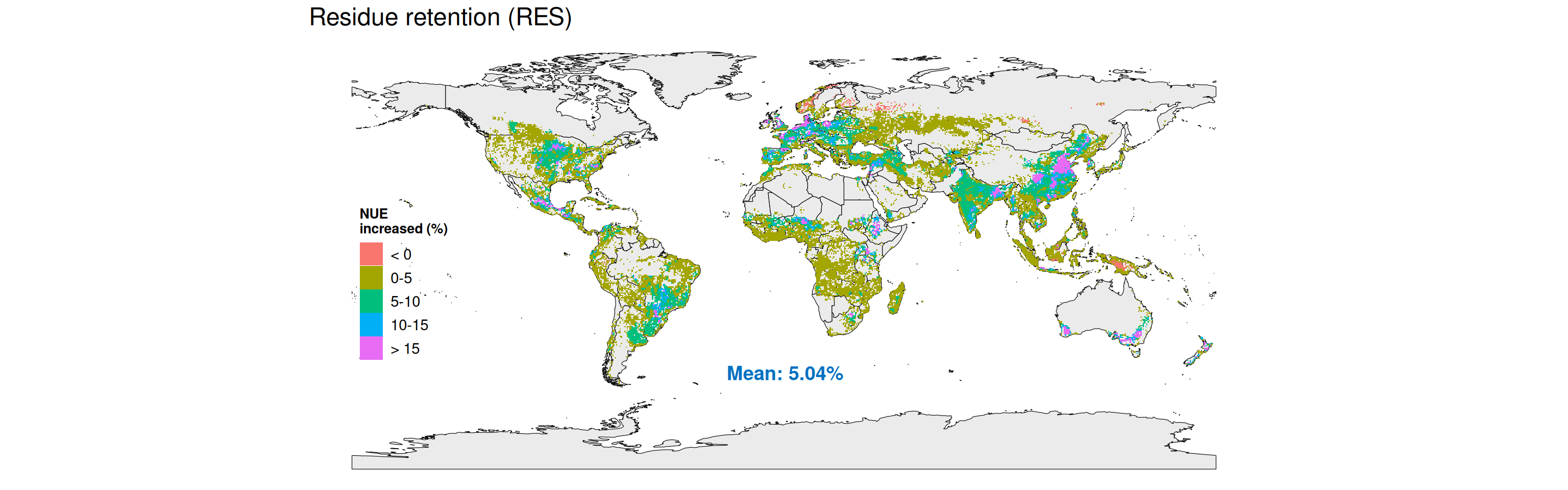
########################################### scenario_SI7 (RES) ######################################################### set themetheme_set(theme_bw())# get the raster to plot r17 <- terra::rast('tif/scenario_SI7.tif')# convert to data.frame r17.p <-as.data.frame(r17,xy=TRUE)# Exclude outliers greater than 70% r17.p <- r17.p[r17.p$improvement <70,]# get base world map world <-ne_countries(scale ="medium", returnclass ="sf")# plot a basic world map plot p17 <-ggplot(data = world) +geom_sf(color ="black", fill ="gray92") +geom_tile(data = r17.p,aes(x=x,y=y, name ='none',fill =cut(improvement,breaks=c(-10,0,5,10,15,1000),labels =c('< 0','0-5','5-10','10-15','> 15') ))) +theme_void() +theme(legend.position =c(0.1,0.45), text =element_text(size =15),legend.background =element_rect(fill =NA,color =NA),panel.border =element_blank()) +labs(fill ='NUE\nincreased (%)') +theme(legend.title =element_text(color ="black", size =10, face ="bold"),legend.text =element_text(color ="black", size =11))+# theme(legend.position = c(0.5, 0.1),# legend.direction = "horizontal")+xlab("Longitude") +ylab("Latitude") +ggtitle("Residue retention (RES)") +#ggtitle("World map", subtitle = "Mean change for scenario 4") +annotate("text",x=0.5,y=-50,label="Mean: 5.04%",size=5, colour="#0070C0",fontface ="bold")+coord_sf(crs =4326)
Warning in geom_tile(data = r17.p, aes(x = x, y = y, name = "none", fill =
cut(improvement, : Ignoring unknown aesthetics: name
p17
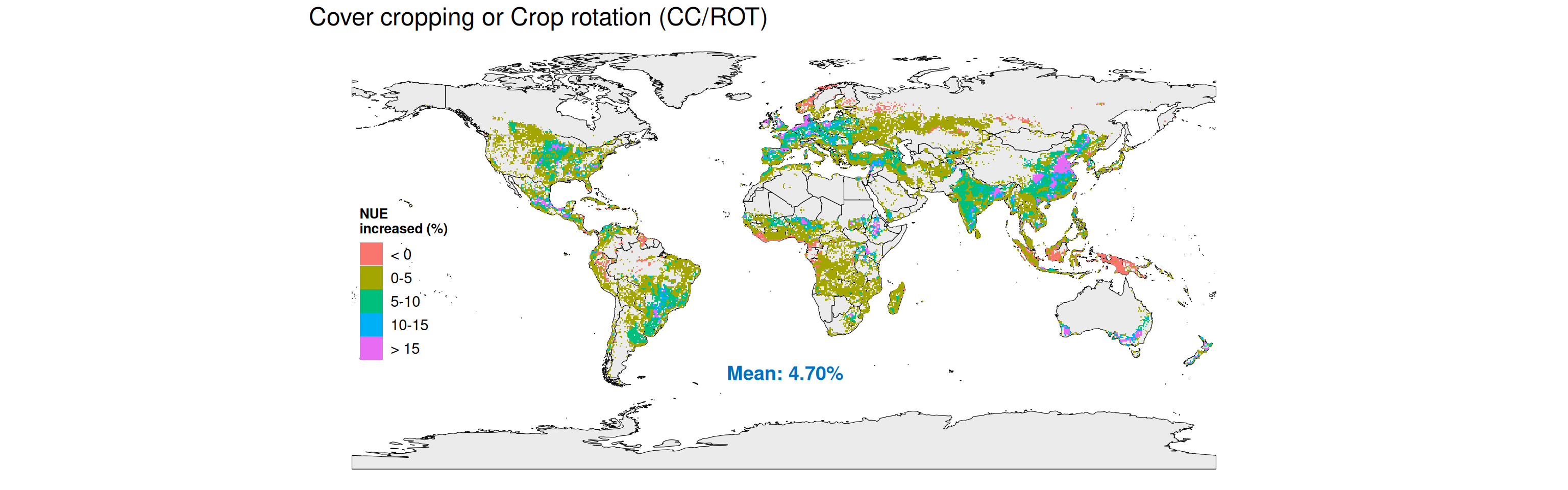
########################################### scenario_SI8 (CC/ROT) ######################################################### set themetheme_set(theme_bw())# get the raster to plot r18 <- terra::rast('tif/scenario_SI8.tif')# convert to data.frame r18.p <-as.data.frame(r18,xy=TRUE)# Exclude outliers greater than 70% r18.p <- r18.p[r18.p$improvement <70,]# get base world map world <-ne_countries(scale ="medium", returnclass ="sf")# plot a basic world map plot p18 <-ggplot(data = world) +geom_sf(color ="black", fill ="gray92") +geom_tile(data = r18.p,aes(x=x,y=y, name ='none',fill =cut(improvement,breaks=c(-10,0,5,10,15,1000),labels =c('< 0','0-5','5-10','10-15','> 15') ))) +theme_void() +theme(legend.position =c(0.1,0.45), text =element_text(size =15),legend.background =element_rect(fill =NA,color =NA),panel.border =element_blank()) +labs(fill ='NUE\nincreased (%)') +theme(legend.title =element_text(color ="black", size =10, face ="bold"),legend.text =element_text(color ="black", size =11))+#theme(legend.position = "none")+xlab("Longitude") +ylab("Latitude") +ggtitle("Cover cropping or Crop rotation (CC/ROT)") +#ggtitle("World map", subtitle = "Mean change for scenario 4") +annotate("text",x=0.5,y=-50,label="Mean: 4.70%",size=5, colour="#0070C0",fontface ="bold")+coord_sf(crs =4326)
Warning in geom_tile(data = r18.p, aes(x = x, y = y, name = "none", fill =
cut(improvement, : Ignoring unknown aesthetics: name
p18
#2*2library(ggpubr)
Attaching package: 'ggpubr'
The following object is masked from 'package:cowplot':

    get_legend
The following object is masked from 'package:terra':

    rotate