11  Tables

# Table 1, Table S5-S7

# Load libraries 
library(data.table)
library(metafor)

Loading required package: Matrix

Loading required package: metadat

Loading required package: numDeriv

Loading the 'metafor' package (version 4.8-0). For an
introduction to the package please type: help(metafor)

library(metagear)

Warning: no DISPLAY variable so Tk is not available

** metagear 0.7, for installing/troubleshooting help see:

**     http://lajeunesse.myweb.usf.edu/metagear/metagear_basic_vignette.html

***** External dependencies check:

***** setup supports GUIs [ FALSE ]

*****    NOTE: Your configuration may still support GUIs,

*****          use the fixes below only after you try

*****          running metagear's abstract_screener().

**

**   Fix for Windows users:

**      Update R (tcltk is now part of all new R builds).

**   Fix for Mac users:

**      Install xQuartz (X11) from https://www.xquartz.org/

***** setup supports data extraction from plots/figures [ FALSE ]

*****       NOTE: EBImage package (Bioconductor) will be installed only

*****             when a figure_* function is used.

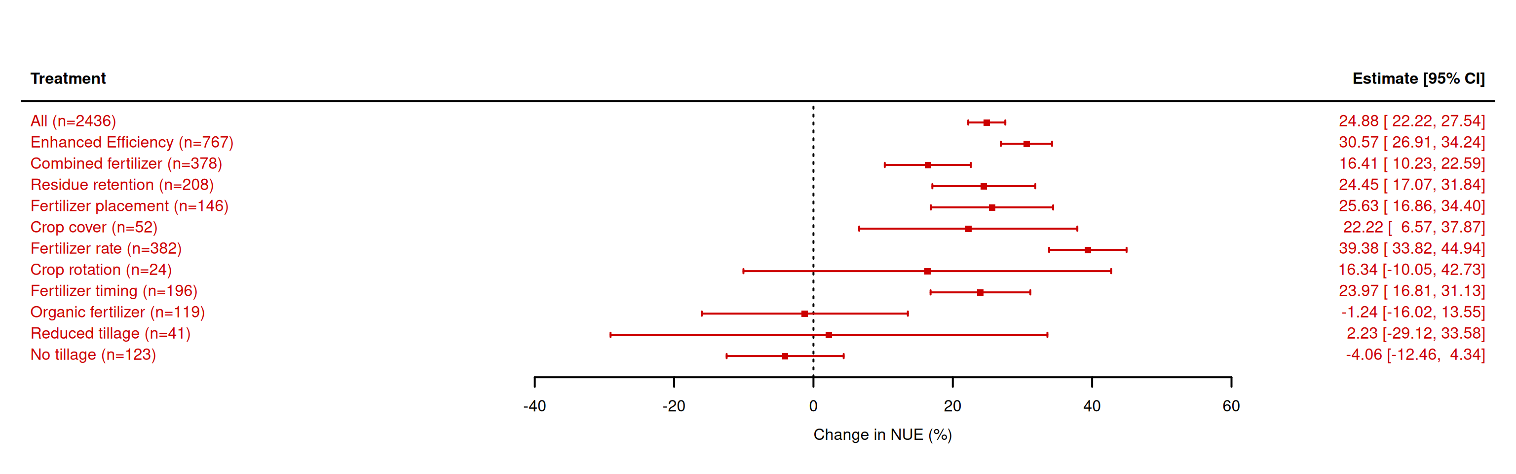
##################################### ROM (metafor) ####################################################
# read data
d1 <- readxl::read_xlsx('Source Data.xlsx',sheet = "Tables")
d1 <- as.data.table(d1)

#Supplement the standard deviation missing value_Common Method
d2<-d1
CV_nuet_bar<-mean(d2$nuet_sd[is.na(d2$nuet_sd)==FALSE]/d2$nuet_mean[is.na(d2$nuet_sd)==FALSE])
d2$nuet_sd[is.na(d2$nuet_sd)==TRUE]<-d2$nuet_mean[is.na(d2$nuet_sd)==TRUE]*1.25*CV_nuet_bar

CV_nuec_bar<-mean(d2$nuec_sd[is.na(d2$nuec_sd)==FALSE]/d2$nuec_mean[is.na(d2$nuec_sd)==FALSE])
d2$nuec_sd[is.na(d2$nuec_sd)==TRUE]<-d2$nuec_mean[is.na(d2$nuec_sd)==TRUE]*1.25*CV_nuec_bar

# clean up column names
d2 <- as.data.table(d2)
setnames(d2,gsub('\\/','_',gsub(' |\\(|\\)','',colnames(d2))))
setnames(d2,tolower(colnames(d2)))

# calculate effect size (NUE)
es21 <- escalc(measure = "ROM", data = d2, 
               m1i = nuet_mean, sd1i = nuet_sd, n1i = replication,
               m2i = nuec_mean, sd2i = nuec_sd, n2i = replication )

# convert to data.tables
d02 <- as.data.table(es21)

# what are the treatments to be assessed
d02.treat <- data.table(treatment =  c('ALL',unique(d02$management)))

# what are labels
d02.treat[treatment=='ALL',desc := 'All']
d02.treat[treatment=='EE',desc := 'Enhanced Efficiency']
d02.treat[treatment=='CF',desc := 'Combined fertilizer']
d02.treat[treatment=='RES',desc := 'Residue retention']
d02.treat[treatment=='RFP',desc := 'Fertilizer placement']
d02.treat[treatment=='RFR',desc := 'Fertilizer rate']
d02.treat[treatment=='ROT',desc := 'Crop rotation']
d02.treat[treatment=='RFT',desc := 'Fertilizer timing']
d02.treat[treatment=='OF',desc := 'Organic fertilizer']
d02.treat[treatment=='RT',desc := 'Reduced tillage']
d02.treat[treatment=='NT',desc := 'No tillage']
d02.treat[treatment=='CC',desc := 'Crop cover']


# a list to store the coefficients
out2 = out3 = list()

# make a for loop to do a main analysis per treatment
for(i in d02.treat$treatment){
  
  if(i=='ALL'){
    
    # run without selection to estimate overall mean
    r_nue <- rma.mv(yi,vi, data=d02,random= list(~ 1|studyid), method="REML",sparse = TRUE)
    
  } else {
    
    # run for selected treatment
    r_nue <- rma.mv(yi,vi, data=d02[management==i,],random= list(~ 1|studyid), method="REML",sparse = TRUE)
    
  }
  
  # save output in a list
  out2[[i]] <- data.table(mean = as.numeric((exp(r_nue$b)-1)*100),
                          se = as.numeric((exp(r_nue$se)-1)*100),
                          pval = round(as.numeric(r_nue$pval),4),
                          label =  paste0(d02.treat[treatment==i,desc],' (n=',r_nue$k,')')
  )
}

# convert lists to vector
out2 <- rbindlist(out2)

# plot for NUE
forest(x = out2$mean, 
       sei = out2$se, 
       slab=out2$label, psize=0.9, cex=1, sortvar=out2$label, xlab="Change in NUE (%)", header="Treatment", col="#CC0000", lwd=2)

Warning in plot.window(...): "sortvar" is not a graphical parameter

Warning in plot.xy(xy, type, ...): "sortvar" is not a graphical parameter

Warning in axis(side = side, at = at, labels = labels, ...): "sortvar" is not a
graphical parameter
Warning in axis(side = side, at = at, labels = labels, ...): "sortvar" is not a
graphical parameter

Warning in box(...): "sortvar" is not a graphical parameter

Warning in title(...): "sortvar" is not a graphical parameter

Warning in int_abline(a = a, b = b, h = h, v = v, untf = untf, ...): "sortvar"
is not a graphical parameter

Warning in segments(...): "sortvar" is not a graphical parameter

Warning in axis(...): "sortvar" is not a graphical parameter

Warning in mtext(...): "sortvar" is not a graphical parameter

Warning in segments(...): "sortvar" is not a graphical parameter
Warning in segments(...): "sortvar" is not a graphical parameter
Warning in segments(...): "sortvar" is not a graphical parameter
Warning in segments(...): "sortvar" is not a graphical parameter
Warning in segments(...): "sortvar" is not a graphical parameter
Warning in segments(...): "sortvar" is not a graphical parameter
Warning in segments(...): "sortvar" is not a graphical parameter
Warning in segments(...): "sortvar" is not a graphical parameter
Warning in segments(...): "sortvar" is not a graphical parameter
Warning in segments(...): "sortvar" is not a graphical parameter
Warning in segments(...): "sortvar" is not a graphical parameter
Warning in segments(...): "sortvar" is not a graphical parameter
Warning in segments(...): "sortvar" is not a graphical parameter
Warning in segments(...): "sortvar" is not a graphical parameter
Warning in segments(...): "sortvar" is not a graphical parameter
Warning in segments(...): "sortvar" is not a graphical parameter
Warning in segments(...): "sortvar" is not a graphical parameter
Warning in segments(...): "sortvar" is not a graphical parameter
Warning in segments(...): "sortvar" is not a graphical parameter
Warning in segments(...): "sortvar" is not a graphical parameter
Warning in segments(...): "sortvar" is not a graphical parameter
Warning in segments(...): "sortvar" is not a graphical parameter
Warning in segments(...): "sortvar" is not a graphical parameter
Warning in segments(...): "sortvar" is not a graphical parameter
Warning in segments(...): "sortvar" is not a graphical parameter
Warning in segments(...): "sortvar" is not a graphical parameter
Warning in segments(...): "sortvar" is not a graphical parameter
Warning in segments(...): "sortvar" is not a graphical parameter
Warning in segments(...): "sortvar" is not a graphical parameter
Warning in segments(...): "sortvar" is not a graphical parameter
Warning in segments(...): "sortvar" is not a graphical parameter
Warning in segments(...): "sortvar" is not a graphical parameter
Warning in segments(...): "sortvar" is not a graphical parameter
Warning in segments(...): "sortvar" is not a graphical parameter
Warning in segments(...): "sortvar" is not a graphical parameter
Warning in segments(...): "sortvar" is not a graphical parameter

Warning in text.default(...): "sortvar" is not a graphical parameter
Warning in text.default(...): "sortvar" is not a graphical parameter

Warning in plot.xy(xy.coords(x, y), type = type, ...): "sortvar" is not a
graphical parameter
Warning in plot.xy(xy.coords(x, y), type = type, ...): "sortvar" is not a
graphical parameter
Warning in plot.xy(xy.coords(x, y), type = type, ...): "sortvar" is not a
graphical parameter
Warning in plot.xy(xy.coords(x, y), type = type, ...): "sortvar" is not a
graphical parameter
Warning in plot.xy(xy.coords(x, y), type = type, ...): "sortvar" is not a
graphical parameter
Warning in plot.xy(xy.coords(x, y), type = type, ...): "sortvar" is not a
graphical parameter
Warning in plot.xy(xy.coords(x, y), type = type, ...): "sortvar" is not a
graphical parameter
Warning in plot.xy(xy.coords(x, y), type = type, ...): "sortvar" is not a
graphical parameter
Warning in plot.xy(xy.coords(x, y), type = type, ...): "sortvar" is not a
graphical parameter
Warning in plot.xy(xy.coords(x, y), type = type, ...): "sortvar" is not a
graphical parameter
Warning in plot.xy(xy.coords(x, y), type = type, ...): "sortvar" is not a
graphical parameter
Warning in plot.xy(xy.coords(x, y), type = type, ...): "sortvar" is not a
graphical parameter

Warning in text.default(...): "sortvar" is not a graphical parameter
Warning in text.default(...): "sortvar" is not a graphical parameter

#publication bias test
#begg’s test
ranktest(out2$mean, sei=out2$se)

Rank Correlation Test for Funnel Plot Asymmetry

Kendall's tau = -0.3333, p = 0.1526

#egger’s test
regtest(out2$mean, out2$se)

Warning: The 'vi' argument should be used to specify sampling variances,
but 'out2$se' sounds like this variable may contain standard
errors (maybe use 'sei=out2$se' instead?).

Regression Test for Funnel Plot Asymmetry

Model:     mixed-effects meta-regression model
Predictor: standard error

Test for Funnel Plot Asymmetry: z = -1.9894, p = 0.0467
Limit Estimate (as sei -> 0):   b =  36.9676 (CI: 17.6886, 56.2465)

# Meta-regression for main factors

# do a first main factor analysis for log response ratio for NUE

# update the missing values for n_dose
d02[is.na(n_dose), n_dose := median(d02$n_dose,na.rm=TRUE)]


# # scale the variables to unit variance
d02[,clay_scaled := scale(clay)]
d02[,soc_scaled := scale(soc)]
d02[,ph_scaled := scale(ph)]
d02[,mat_scaled := scale(mat)]
d02[,map_scaled := scale(map)]
d02[,n_dose_scaled := scale(n_dose)]

# what are the factors to be evaluated
var.site <- c('mat_scaled','map_scaled','clay_scaled','soc_scaled','ph_scaled')
var.crop <- c('g_crop_type','n_dose_scaled')
var.trea <- c('fertilizer_type', 'crop_residue', 'tillage', 'cover_crop_and_crop_rotation', 'fertilizer_strategy')

# i select only one example

# the columns to be assessed
var.sel <- c(var.trea,var.crop,var.site)

# run without a main factor selection to estimate overall mean
r_nue_0 <- rma.mv(yi,vi, data = d02,random= list(~ 1|studyid), method="REML",sparse = TRUE)

# objects to store the effects per factor as wel summary stats of the meta-analytical models
out1.est = out1.sum = list()

# evaluate the impact of treatment (column tillage) on NUE given site properties
for(i in var.sel){
  
  # check whether the column is a numeric or categorical variable
  vartype = is.character(d02[,get(i)])
  
  # run with the main factor treatment
  if(vartype == TRUE){
    
    # run a meta-regression model for main categorial variable
    r_nue_1 <- rma.mv(yi,vi, 
                      mods = ~factor(varsel)-1, 
                      data = d02[,.(yi,vi,studyid,varsel = get(i))],
                      random = list(~ 1|studyid), method="REML",sparse = TRUE)
    
  } else {
    
    # run a meta-regression model for main numerical variable
    r_nue_1 <- rma.mv(yi,vi, 
                      mods = ~varsel, 
                      data = d02[,.(yi,vi,studyid,varsel = get(i))],
                      random = list(~ 1|studyid), method="REML",sparse = TRUE)
  }
  
  # save output in a list: the estimated impact of the explanatory variable
  out1.est[[i]] <- data.table(var = i,
                              varname = gsub('factor\\(varsel\\)','',rownames(r_nue_1$b)),
                              mean = round(as.numeric(r_nue_1$b),3),
                              se = round(as.numeric(r_nue_1$se),3),
                              ci.lb = round(as.numeric(r_nue_1$ci.lb),3),
                              ci.ub = round(as.numeric(r_nue_1$ci.ub),3),
                              pval = round(as.numeric(r_nue_1$pval),3))
  
  # save output in a list: the summary stats collected
  out1.sum[[i]] <- data.table(var = i,
                              AIC = r_nue_1$fit.stats[4,2],
                              ll = r_nue_1$fit.stats[1,2],
                              ll_impr = round(100 * (1-r_nue_1$fit.stats[1,2]/r_nue_0$fit.stats[1,2]),2),
                              r2_impr = round(100*max(0,(sum(r_nue_0$sigma2)-sum(r_nue_1$sigma2))/sum(r_nue_0$sigma2)),2),
                              pval = round(anova(r_nue_1,r_nue_0)$pval,3)
  )
  
}

Warning: REML comparisons not meaningful for models with different fixed effects
(use 'refit=TRUE' to refit both models based on ML estimation).

Warning: REML comparisons not meaningful for models with different fixed effects
(use 'refit=TRUE' to refit both models based on ML estimation).
Warning: REML comparisons not meaningful for models with different fixed effects
(use 'refit=TRUE' to refit both models based on ML estimation).
Warning: REML comparisons not meaningful for models with different fixed effects
(use 'refit=TRUE' to refit both models based on ML estimation).
Warning: REML comparisons not meaningful for models with different fixed effects
(use 'refit=TRUE' to refit both models based on ML estimation).
Warning: REML comparisons not meaningful for models with different fixed effects
(use 'refit=TRUE' to refit both models based on ML estimation).
Warning: REML comparisons not meaningful for models with different fixed effects
(use 'refit=TRUE' to refit both models based on ML estimation).
Warning: REML comparisons not meaningful for models with different fixed effects
(use 'refit=TRUE' to refit both models based on ML estimation).
Warning: REML comparisons not meaningful for models with different fixed effects
(use 'refit=TRUE' to refit both models based on ML estimation).
Warning: REML comparisons not meaningful for models with different fixed effects
(use 'refit=TRUE' to refit both models based on ML estimation).
Warning: REML comparisons not meaningful for models with different fixed effects
(use 'refit=TRUE' to refit both models based on ML estimation).
Warning: REML comparisons not meaningful for models with different fixed effects
(use 'refit=TRUE' to refit both models based on ML estimation).

# merge output into a data.table
out1.sum <- rbindlist(out1.sum)
out1.est <- rbindlist(out1.est)

# Meta-regression for main factors with interactions

# make a function to extract relevant model statistics
estats <- function(model_new,model_base){
  out <- data.table(AIC = model_new$fit.stats[4,2],
                    ll = model_new$fit.stats[1,2],
                    ll_impr = round(100 * (1-model_new$fit.stats[1,2]/model_base$fit.stats[1,2]),2),
                    r2_impr = round(100*max(0,(sum(model_base$sigma2)-sum(model_new$sigma2))/sum(model_base$sigma2)),2),
                    pval = round(anova(r_nue_1,r_nue_0)$pval,3))
  return(out)
}

d02[tillage=='reduced', tillage := 'no-till']

d02[,fertilizer_type := factor(fertilizer_type,
                               levels = c('mineral','organic', 'combined','enhanced'))] 
d02[,fertilizer_strategy := factor(fertilizer_strategy,
                                   levels = c("conventional", "placement","rate","timing"))]
d02[,g_crop_type := factor(g_crop_type,
                           levels = c('maize','wheat','rice'))]

d4 <- copy(d02)

d4[,r4pl := fifelse(fertilizer_strategy=='placement','yes','no')]
d4[,r4ti := fifelse(fertilizer_strategy=='timing','yes','no')]
d4[,r4do := fifelse(fertilizer_strategy=='rate','yes','no')]
d4[,ctm := fifelse(g_crop_type=='maize','yes','no')]
d4[,ctw := fifelse(g_crop_type=='wheat','yes','no')]
d4[,ctr := fifelse(g_crop_type=='rice','yes','no')]
d4[,ndose2 := scale(n_dose^2)]


# run without a main factor selection to estimate overall mean
r_nue_0 <- rma.mv(yi,vi, data = d02,random= list(~ 1|studyid), method="REML",sparse = TRUE)

r_nue_4 <- rma.mv(yi,vi,
                  mods = ~fertilizer_type + r4pl + r4ti + r4do + crop_residue + tillage +
                    cover_crop_and_crop_rotation + n_dose_scaled + clay_scaled + ph_scaled + map_scaled + mat_scaled + soc_scaled+
                    soc_scaled : n_dose_scaled + ctm:r4pl + ctm + ctw + ctr + ctm:mat_scaled  + ndose2 -1,
                  data = d4,
                  random = list(~ 1|studyid), method="REML",sparse = TRUE)

Warning: Redundant predictors dropped from the model.

# show stats and improvements
out = estats(model_new = r_nue_4,model_base = r_nue_0)

Warning: REML comparisons not meaningful for models with different fixed effects
(use 'refit=TRUE' to refit both models based on ML estimation).

print(paste0('model improved the log likelyhood with ',round(out$ll_impr,1),'%'))

[1] "model improved the log likelyhood with 43.4%"

summary(r_nue_4)

Multivariate Meta-Analysis Model (k = 2436; method: REML)

     logLik     Deviance          AIC          BIC         AICc   
-22948.6157   45897.2315   45943.2315   46076.3794   45943.6934   

Variance Components:

            estim    sqrt  nlvls  fixed   factor 
sigma^2    0.1230  0.3507    408     no  studyid 

Test for Residual Heterogeneity:
QE(df = 2414) = 80253.7924, p-val < .0001

Test of Moderators (coefficients 1:22):
QM(df = 22) = 35448.6633, p-val < .0001

Model Results:

                                 estimate      se       zval    pval    ci.lb 
fertilizer_typemineral             0.0956  0.0195     4.9015  <.0001   0.0574 
fertilizer_typeorganic             0.1771  0.0210     8.4374  <.0001   0.1359 
fertilizer_typecombined            0.2129  0.0206    10.3357  <.0001   0.1725 
fertilizer_typeenhanced            0.3495  0.0190    18.3681  <.0001   0.3122 
r4plyes                            0.1419  0.0182     7.8122  <.0001   0.1063 
r4tiyes                            0.2036  0.0137    14.8831  <.0001   0.1768 
r4doyes                            0.1827  0.0115    15.8944  <.0001   0.1602 
crop_residueyes                    0.0725  0.0127     5.7246  <.0001   0.0477 
tillageno-till                    -0.0638  0.0144    -4.4467  <.0001  -0.0920 
cover_crop_and_crop_rotationyes    0.1317  0.0265     4.9758  <.0001   0.0798 
n_dose_scaled                     -1.1786  0.0088  -134.5849  <.0001  -1.1957 
clay_scaled                       -0.0706  0.0115    -6.1567  <.0001  -0.0930 
ph_scaled                          0.0522  0.0142     3.6613  0.0003   0.0242 
map_scaled                         0.1259  0.0191     6.5807  <.0001   0.0884 
mat_scaled                        -0.0723  0.0176    -4.1005  <.0001  -0.1069 
soc_scaled                         0.0626  0.0113     5.5641  <.0001   0.0406 
ctmyes                            -0.0049  0.0115    -0.4295  0.6676  -0.0274 
ctwyes                            -0.0353  0.0016   -21.7282  <.0001  -0.0385 
ndose2                             1.1200  0.0090   124.6274  <.0001   1.1024 
n_dose_scaled:soc_scaled           0.0627  0.0040    15.6320  <.0001   0.0548 
r4plyes:ctmyes                    -0.3404  0.0211   -16.1257  <.0001  -0.3818 
mat_scaled:ctmyes                  0.1322  0.0231     5.7221  <.0001   0.0869 
                                   ci.ub      
fertilizer_typemineral            0.1338  *** 
fertilizer_typeorganic            0.2182  *** 
fertilizer_typecombined           0.2532  *** 
fertilizer_typeenhanced           0.3867  *** 
r4plyes                           0.1774  *** 
r4tiyes                           0.2304  *** 
r4doyes                           0.2053  *** 
crop_residueyes                   0.0973  *** 
tillageno-till                   -0.0357  *** 
cover_crop_and_crop_rotationyes   0.1836  *** 
n_dose_scaled                    -1.1614  *** 
clay_scaled                      -0.0481  *** 
ph_scaled                         0.0801  *** 
map_scaled                        0.1634  *** 
mat_scaled                       -0.0378  *** 
soc_scaled                        0.0847  *** 
ctmyes                            0.0175      
ctwyes                           -0.0321  *** 
ndose2                            1.1377  *** 
n_dose_scaled:soc_scaled          0.0706  *** 
r4plyes:ctmyes                   -0.2991  *** 
mat_scaled:ctmyes                 0.1775  *** 

---
Signif. codes:  0 '***' 0.001 '**' 0.01 '*' 0.05 '.' 0.1 ' ' 1

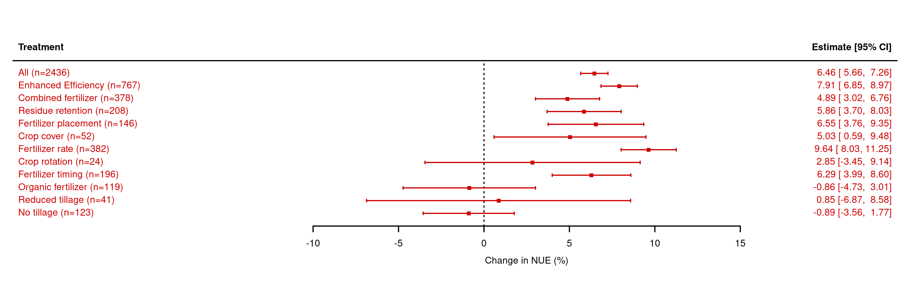
k <- r_nue_4$k
wi <- 1/r_nue_4$vi
vt <- (k-1) / (sum(wi) - sum(wi^2)/sum(wi))
PR2 <- r_nue_0$sigma2 / (sum(r_nue_4$sigma2) + vt)


##################################### MD (metafor) ####################################################
# read data
d1 <- readxl::read_xlsx('Source Data.xlsx',sheet = "Tables")
d1 <- as.data.table(d1)

# Supplement the SD when missing
d2<-d1
CV_nuet_bar<-mean(d2$nuet_sd[is.na(d2$nuet_sd)==FALSE]/d2$nuet_mean[is.na(d2$nuet_sd)==FALSE])
d2$nuet_sd[is.na(d2$nuet_sd)==TRUE]<-d2$nuet_mean[is.na(d2$nuet_sd)==TRUE]*1.25*CV_nuet_bar

CV_nuec_bar<-mean(d2$nuec_sd[is.na(d2$nuec_sd)==FALSE]/d2$nuec_mean[is.na(d2$nuec_sd)==FALSE])
d2$nuec_sd[is.na(d2$nuec_sd)==TRUE]<-d2$nuec_mean[is.na(d2$nuec_sd)==TRUE]*1.25*CV_nuec_bar

# clean up column names
d2 <- as.data.table(d2)
setnames(d2,gsub('\\/','_',gsub(' |\\(|\\)','',colnames(d2))))
setnames(d2,tolower(colnames(d2)))

# calculate effect size (MD)
es21 <- escalc(measure = "MD", data = d2, 
               m1i = nuet_mean, sd1i = nuet_sd, n1i = replication,
               m2i = nuec_mean, sd2i = nuec_sd, n2i = replication )

# convert to data.tables
d02 <- as.data.table(es21)

# what are the treatments to be assessed
d02.treat <- data.table(treatment =  c('ALL',unique(d02$management)))

# what are labels
d02.treat[treatment=='ALL',desc := 'All']
d02.treat[treatment=='EE',desc := 'Enhanced Efficiency']
d02.treat[treatment=='CF',desc := 'Combined fertilizer']
d02.treat[treatment=='RES',desc := 'Residue retention']
d02.treat[treatment=='RFP',desc := 'Fertilizer placement']
d02.treat[treatment=='RFR',desc := 'Fertilizer rate']
d02.treat[treatment=='ROT',desc := 'Crop rotation']
d02.treat[treatment=='RFT',desc := 'Fertilizer timing']
d02.treat[treatment=='OF',desc := 'Organic fertilizer']
d02.treat[treatment=='RT',desc := 'Reduced tillage']
d02.treat[treatment=='NT',desc := 'No tillage']
d02.treat[treatment=='CC',desc := 'Crop cover']

# a list to store the coefficients
out2 = out3 = list()

# make a for loop to do a main analysis per treatment
for(i in d02.treat$treatment){
  
  if(i=='ALL'){
    
    # run without selection to estimate overall mean
    r_nue <- rma.mv(yi,vi, data=d02,random= list(~ 1|studyid), method="REML",sparse = TRUE)
    
  } else {
    
    # run for selected treatment
    r_nue <- rma.mv(yi,vi, data=d02[management==i,],random= list(~ 1|studyid), method="REML",sparse = TRUE)
    
  }
  
  # save output in a list
  out2[[i]] <- data.table(mean = as.numeric(r_nue$b),
                          se = as.numeric(r_nue$se),
                          label =  paste0(d02.treat[treatment==i,desc],' (n=',r_nue$k,')')
  )
}

# convert lists to vector
out2 <- rbindlist(out2)

# plot for NUE
forest(x = out2$mean,
       sei = out2$se, slab=out2$label, psize=0.9, cex=1, sortvar=out2$label, xlab="Change in NUE (%)", header="Treatment", col="#CC0000", lwd=2)

Warning in plot.window(...): "sortvar" is not a graphical parameter

Warning in plot.xy(xy, type, ...): "sortvar" is not a graphical parameter

Warning in axis(side = side, at = at, labels = labels, ...): "sortvar" is not a
graphical parameter
Warning in axis(side = side, at = at, labels = labels, ...): "sortvar" is not a
graphical parameter

Warning in box(...): "sortvar" is not a graphical parameter

Warning in title(...): "sortvar" is not a graphical parameter

Warning in int_abline(a = a, b = b, h = h, v = v, untf = untf, ...): "sortvar"
is not a graphical parameter

Warning in segments(...): "sortvar" is not a graphical parameter

Warning in axis(...): "sortvar" is not a graphical parameter

Warning in mtext(...): "sortvar" is not a graphical parameter

Warning in segments(...): "sortvar" is not a graphical parameter
Warning in segments(...): "sortvar" is not a graphical parameter
Warning in segments(...): "sortvar" is not a graphical parameter
Warning in segments(...): "sortvar" is not a graphical parameter
Warning in segments(...): "sortvar" is not a graphical parameter
Warning in segments(...): "sortvar" is not a graphical parameter
Warning in segments(...): "sortvar" is not a graphical parameter
Warning in segments(...): "sortvar" is not a graphical parameter
Warning in segments(...): "sortvar" is not a graphical parameter
Warning in segments(...): "sortvar" is not a graphical parameter
Warning in segments(...): "sortvar" is not a graphical parameter
Warning in segments(...): "sortvar" is not a graphical parameter
Warning in segments(...): "sortvar" is not a graphical parameter
Warning in segments(...): "sortvar" is not a graphical parameter
Warning in segments(...): "sortvar" is not a graphical parameter
Warning in segments(...): "sortvar" is not a graphical parameter
Warning in segments(...): "sortvar" is not a graphical parameter
Warning in segments(...): "sortvar" is not a graphical parameter
Warning in segments(...): "sortvar" is not a graphical parameter
Warning in segments(...): "sortvar" is not a graphical parameter
Warning in segments(...): "sortvar" is not a graphical parameter
Warning in segments(...): "sortvar" is not a graphical parameter
Warning in segments(...): "sortvar" is not a graphical parameter
Warning in segments(...): "sortvar" is not a graphical parameter
Warning in segments(...): "sortvar" is not a graphical parameter
Warning in segments(...): "sortvar" is not a graphical parameter
Warning in segments(...): "sortvar" is not a graphical parameter
Warning in segments(...): "sortvar" is not a graphical parameter
Warning in segments(...): "sortvar" is not a graphical parameter
Warning in segments(...): "sortvar" is not a graphical parameter
Warning in segments(...): "sortvar" is not a graphical parameter
Warning in segments(...): "sortvar" is not a graphical parameter
Warning in segments(...): "sortvar" is not a graphical parameter
Warning in segments(...): "sortvar" is not a graphical parameter
Warning in segments(...): "sortvar" is not a graphical parameter
Warning in segments(...): "sortvar" is not a graphical parameter

Warning in text.default(...): "sortvar" is not a graphical parameter
Warning in text.default(...): "sortvar" is not a graphical parameter

Warning in plot.xy(xy.coords(x, y), type = type, ...): "sortvar" is not a
graphical parameter
Warning in plot.xy(xy.coords(x, y), type = type, ...): "sortvar" is not a
graphical parameter
Warning in plot.xy(xy.coords(x, y), type = type, ...): "sortvar" is not a
graphical parameter
Warning in plot.xy(xy.coords(x, y), type = type, ...): "sortvar" is not a
graphical parameter
Warning in plot.xy(xy.coords(x, y), type = type, ...): "sortvar" is not a
graphical parameter
Warning in plot.xy(xy.coords(x, y), type = type, ...): "sortvar" is not a
graphical parameter
Warning in plot.xy(xy.coords(x, y), type = type, ...): "sortvar" is not a
graphical parameter
Warning in plot.xy(xy.coords(x, y), type = type, ...): "sortvar" is not a
graphical parameter
Warning in plot.xy(xy.coords(x, y), type = type, ...): "sortvar" is not a
graphical parameter
Warning in plot.xy(xy.coords(x, y), type = type, ...): "sortvar" is not a
graphical parameter
Warning in plot.xy(xy.coords(x, y), type = type, ...): "sortvar" is not a
graphical parameter
Warning in plot.xy(xy.coords(x, y), type = type, ...): "sortvar" is not a
graphical parameter

Warning in text.default(...): "sortvar" is not a graphical parameter
Warning in text.default(...): "sortvar" is not a graphical parameter

#publication bias test

#begg’s test
ranktest(out2$mean, out2$se)

Rank Correlation Test for Funnel Plot Asymmetry

Kendall's tau = -0.4545, p = 0.0447

#egger’s test
regtest(out2$mean, out2$se)

Regression Test for Funnel Plot Asymmetry

Model:     mixed-effects meta-regression model
Predictor: standard error

Test for Funnel Plot Asymmetry: z = -2.4494, p = 0.0143
Limit Estimate (as sei -> 0):   b =  10.9299 (CI: 5.7644, 16.0955)

# Meta-regression for main factors
# do a first main factor analysis for log response ratio for NUE

# update the missing values for n_dose and p2o5_dose (as example)
d02[is.na(n_dose), n_dose := median(d02$n_dose,na.rm=TRUE)]

# scale the variables to unit variance
d02[,clay_scaled := scale(clay)]
d02[,soc_scaled := scale(soc)]
d02[,ph_scaled := scale(ph)]
d02[,mat_scaled := scale(mat)]
d02[,map_scaled := scale(map)]
d02[,n_dose_scaled := scale(n_dose)]

# what are the factors to be evaluated
var.site <- c('mat_scaled','map_scaled','clay_scaled','soc_scaled','ph_scaled')
var.crop <- c('g_crop_type','n_dose_scaled')

var.trea <- c('fertilizer_type', 'crop_residue', 'tillage', 'cover_crop_and_crop_rotation', 'fertilizer_strategy')

# i select only one example

# the columns to be assessed
var.sel <- c(var.trea,var.crop,var.site)

# run without a main factor selection to estimate overall mean
r_nue_0 <- rma.mv(yi,vi, data = d02,random= list(~ 1|studyid), method="REML",sparse = TRUE)

# objects to store the effects per factor as wel summary stats of the meta-analytical models
out1.est = out1.sum = list()

# evaluate the impact of treatment (column tillage) on NUE given site properties
for(i in var.sel){
  
  # check whether the column is a numeric or categorical variable
  vartype = is.character(d02[,get(i)])
  
  # run with the main factor treatment
  if(vartype == TRUE){
    
    # run a meta-regression model for main categorial variable
    r_nue_1 <- rma.mv(yi,vi, 
                      mods = ~factor(varsel)-1, 
                      data = d02[,.(yi,vi,studyid,varsel = get(i))],
                      random = list(~ 1|studyid), method="REML",sparse = TRUE)
    
  } else {
    
    # run a meta-regression model for main numerical variable
    r_nue_1 <- rma.mv(yi,vi, 
                      mods = ~varsel, 
                      data = d02[,.(yi,vi,studyid,varsel = get(i))],
                      random = list(~ 1|studyid), method="REML",sparse = TRUE)
  }
  
  # save output in a list: the estimated impact of the explanatory variable
  out1.est[[i]] <- data.table(var = i,
                              varname = gsub('factor\\(varsel\\)','',rownames(r_nue_1$b)),
                              mean = round(as.numeric(r_nue_1$b),3),
                              se = round(as.numeric(r_nue_1$se),3),
                              ci.lb = round(as.numeric(r_nue_1$ci.lb),3),
                              ci.ub = round(as.numeric(r_nue_1$ci.ub),3),
                              pval = round(as.numeric(r_nue_1$pval),3))
  
  # save output in a list: the summary stats collected
  out1.sum[[i]] <- data.table(var = i,
                              AIC = r_nue_1$fit.stats[4,2],
                              ll = r_nue_1$fit.stats[1,2],
                              ll_impr = round(100 * (1-r_nue_1$fit.stats[1,2]/r_nue_0$fit.stats[1,2]),2),
                              r2_impr = round(100*max(0,(sum(r_nue_0$sigma2)-sum(r_nue_1$sigma2))/sum(r_nue_0$sigma2)),2),
                              pval = round(anova(r_nue_1,r_nue_0)$pval,3)
  )
  
}

Warning: REML comparisons not meaningful for models with different fixed effects
(use 'refit=TRUE' to refit both models based on ML estimation).

Warning: REML comparisons not meaningful for models with different fixed effects
(use 'refit=TRUE' to refit both models based on ML estimation).
Warning: REML comparisons not meaningful for models with different fixed effects
(use 'refit=TRUE' to refit both models based on ML estimation).
Warning: REML comparisons not meaningful for models with different fixed effects
(use 'refit=TRUE' to refit both models based on ML estimation).
Warning: REML comparisons not meaningful for models with different fixed effects
(use 'refit=TRUE' to refit both models based on ML estimation).
Warning: REML comparisons not meaningful for models with different fixed effects
(use 'refit=TRUE' to refit both models based on ML estimation).
Warning: REML comparisons not meaningful for models with different fixed effects
(use 'refit=TRUE' to refit both models based on ML estimation).
Warning: REML comparisons not meaningful for models with different fixed effects
(use 'refit=TRUE' to refit both models based on ML estimation).
Warning: REML comparisons not meaningful for models with different fixed effects
(use 'refit=TRUE' to refit both models based on ML estimation).
Warning: REML comparisons not meaningful for models with different fixed effects
(use 'refit=TRUE' to refit both models based on ML estimation).
Warning: REML comparisons not meaningful for models with different fixed effects
(use 'refit=TRUE' to refit both models based on ML estimation).
Warning: REML comparisons not meaningful for models with different fixed effects
(use 'refit=TRUE' to refit both models based on ML estimation).

# merge output into a data.table
out1.sum <- rbindlist(out1.sum)
out1.est <- rbindlist(out1.est)

# Meta-regression for main factors with interactions

# make a function to extract relevant model statistics
estats <- function(model_new,model_base){
  out <- data.table(AIC = model_new$fit.stats[4,2],
                    ll = model_new$fit.stats[1,2],
                    ll_impr = round(100 * (1-model_new$fit.stats[1,2]/model_base$fit.stats[1,2]),2),
                    r2_impr = round(100*max(0,(sum(model_base$sigma2)-sum(model_new$sigma2))/sum(model_base$sigma2)),2),
                    pval = round(anova(r_nue_1,r_nue_0)$pval,3))
  return(out)
}

# update the database (it looks like typos)

d02[tillage=='reduced', tillage := 'no-till']


d02[,fertilizer_type := factor(fertilizer_type,
                               levels = c('mineral','organic', 'combined','enhanced'))]
d02[,fertilizer_strategy := factor(fertilizer_strategy,
                                   levels = c("conventional", "placement","rate","timing"))]
d02[,g_crop_type := factor(g_crop_type,
                           levels = c('maize','wheat','rice'))]

d4 <- copy(d02)

d4[,r4pl := fifelse(fertilizer_strategy=='placement','yes','no')]
d4[,r4ti := fifelse(fertilizer_strategy=='timing','yes','no')]
d4[,r4do := fifelse(fertilizer_strategy=='rate','yes','no')]
d4[,ctm := fifelse(g_crop_type=='maize','yes','no')]
d4[,ctw := fifelse(g_crop_type=='wheat','yes','no')]
d4[,ctr := fifelse(g_crop_type=='rice','yes','no')]
d4[,ndose2 := scale(n_dose^2)]

# run without a main factor selection to estimate overall mean
r_nue_0 <- rma.mv(yi,vi, data = d02,random= list(~ 1|studyid), method="REML",sparse = TRUE)

r_nue_4 <- rma.mv(yi,vi,
                  mods = ~fertilizer_type + r4pl + r4ti + r4do + crop_residue + tillage +
                    cover_crop_and_crop_rotation + n_dose_scaled + clay_scaled + ph_scaled + map_scaled + mat_scaled + soc_scaled +
                    soc_scaled : n_dose_scaled + ctm:r4pl + ctm + ctw + ctr + ctm:mat_scaled  + ndose2 -1,
                  data = d4,
                  random = list(~ 1|studyid), method="REML",sparse = TRUE)

Warning: Redundant predictors dropped from the model.

# show stats and improvements
out = estats(model_new = r_nue_4,model_base = r_nue_0)

Warning: REML comparisons not meaningful for models with different fixed effects
(use 'refit=TRUE' to refit both models based on ML estimation).

print(paste0('model improved the log likelyhood with ',round(out$ll_impr,1),'%'))

[1] "model improved the log likelyhood with 32.9%"

summary(r_nue_4)

Multivariate Meta-Analysis Model (k = 2436; method: REML)

     logLik     Deviance          AIC          BIC         AICc   
-27694.8843   55389.7685   55435.7685   55568.9165   55436.2305   

Variance Components:

             estim    sqrt  nlvls  fixed   factor 
sigma^2    96.1315  9.8047    408     no  studyid 

Test for Residual Heterogeneity:
QE(df = 2414) = 63270.0073, p-val < .0001

Test of Moderators (coefficients 1:22):
QM(df = 22) = 27221.4896, p-val < .0001

Model Results:

                                 estimate      se       zval    pval     ci.lb 
fertilizer_typemineral             4.8150  0.5415     8.8915  <.0001    3.7536 
fertilizer_typeorganic             3.7867  0.6204     6.1034  <.0001    2.5707 
fertilizer_typecombined            7.5767  0.5854    12.9422  <.0001    6.4293 
fertilizer_typeenhanced            8.0954  0.5367    15.0826  <.0001    7.0434 
r4plyes                            1.8479  0.5348     3.4555  0.0005    0.7998 
r4tiyes                            3.2728  0.3493     9.3704  <.0001    2.5882 
r4doyes                            4.3411  0.3541    12.2586  <.0001    3.6470 
crop_residueyes                    1.8930  0.3415     5.5435  <.0001    1.2237 
tillageno-till                    -2.8625  0.4299    -6.6585  <.0001   -3.7050 
cover_crop_and_crop_rotationyes    1.5543  0.5517     2.8174  0.0048    0.4730 
n_dose_scaled                    -30.1474  0.2784  -108.3012  <.0001  -30.6930 
clay_scaled                       -2.2753  0.3245    -7.0124  <.0001   -2.9113 
ph_scaled                          0.2732  0.3074     0.8887  0.3742   -0.3293 
map_scaled                         0.9656  0.3854     2.5056  0.0122    0.2103 
mat_scaled                        -0.4163  0.4925    -0.8453  0.3979   -1.3817 
soc_scaled                         1.1541  0.3561     3.2407  0.0012    0.4561 
ctmyes                            -0.7213  0.3158    -2.2839  0.0224   -1.3403 
ctwyes                             0.1205  0.0633     1.9030  0.0570   -0.0036 
ndose2                            27.9200  0.2822    98.9533  <.0001   27.3670 
n_dose_scaled:soc_scaled           0.4221  0.1229     3.4338  0.0006    0.1812 
r4plyes:ctmyes                    -3.0466  0.5610    -5.4310  <.0001   -4.1461 
mat_scaled:ctmyes                  2.3939  0.6452     3.7104  0.0002    1.1294 
                                    ci.ub      
fertilizer_typemineral             5.8763  *** 
fertilizer_typeorganic             5.0027  *** 
fertilizer_typecombined            8.7242  *** 
fertilizer_typeenhanced            9.1473  *** 
r4plyes                            2.8960  *** 
r4tiyes                            3.9573  *** 
r4doyes                            5.0351  *** 
crop_residueyes                    2.5623  *** 
tillageno-till                    -2.0199  *** 
cover_crop_and_crop_rotationyes    2.6355   ** 
n_dose_scaled                    -29.6018  *** 
clay_scaled                       -1.6394  *** 
ph_scaled                          0.8757      
map_scaled                         1.7209    * 
mat_scaled                         0.5490      
soc_scaled                         1.8521   ** 
ctmyes                            -0.1023    * 
ctwyes                             0.2445    . 
ndose2                            28.4731  *** 
n_dose_scaled:soc_scaled           0.6631  *** 
r4plyes:ctmyes                    -1.9471  *** 
mat_scaled:ctmyes                  3.6584  *** 

---
Signif. codes:  0 '***' 0.001 '**' 0.01 '*' 0.05 '.' 0.1 ' ' 1

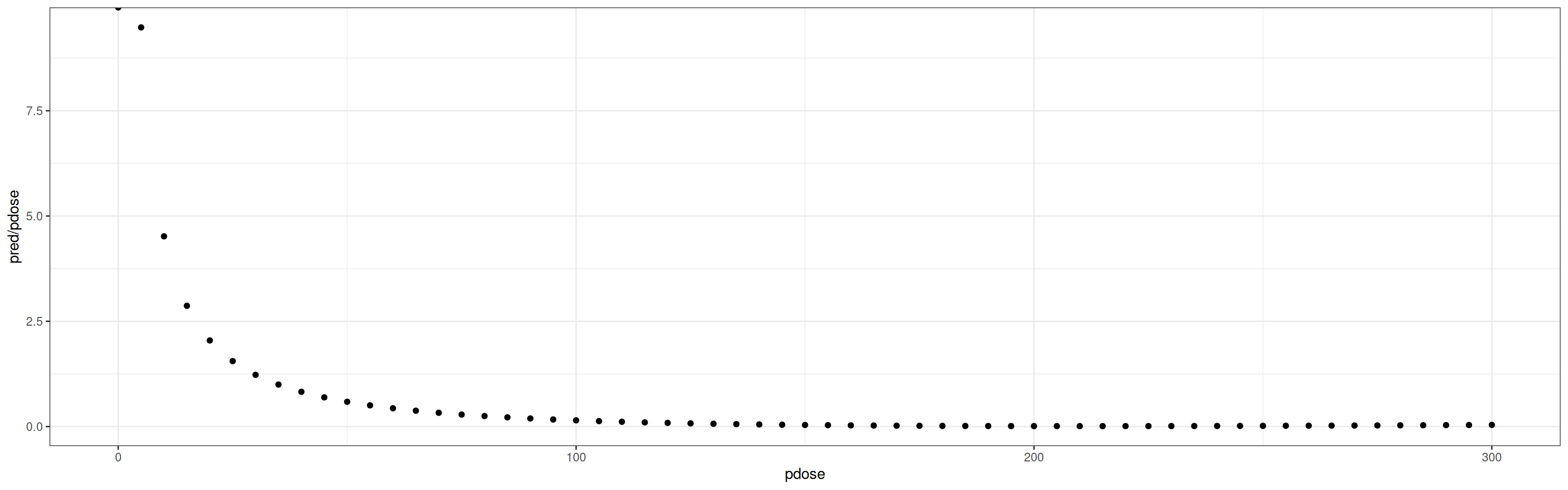
k <- r_nue_4$k
wi <- 1/r_nue_4$vi
vt <- (k-1) / (sum(wi) - sum(wi^2)/sum(wi))
PR2 <- r_nue_0$sigma2 / (sum(r_nue_4$sigma2) + vt)

# Model predictions
ms = predict(r_nue_4,addx=T)         

# this is the order of input variables needed for model predictions (=newmods in predict function)
cols <- colnames(ms$X)

# make a prediction data.table
dt.pred <- as.data.table(t(ms$X[1,]))

# set all variables to 0
dt.pred[,c(cols) := 0,]

# add the series of N dose
dt.pred <- cbind(dt.pred,ndose = seq(0,300,5))
dt.pred[,n_dose_scaled := (ndose - mean(d4$n_dose))/sd(d4$n_dose)]
dt.pred[,ndose2 := (ndose^2 - mean(d4$n_dose^2))/sd(d4$n_dose^2) ]

# update the enhanced column (set to 1, all others are zero = non applicable)
dt.pred[, fertilizer_typeenhanced := 1]

# remove ndose
dt.pred[,ndose := NULL]

# predict for EE and variable N dose
m2 = predict(r_nue_4,newmods=as.matrix(dt.pred),addx=T) 

m2 = as.data.frame(m2)

# plot prediction (now without confidence)

# get the original Ndose here
m2 = as.data.table(m2)
m2[,pdose := seq(0,300,5)]

mean(d4$n_dose)

[1] 172.9166

m2[pdose >170 & pdose<=180,][1]

       pred        se    ci.lb    ci.ub     pi.lb    pi.ub
      <num>     <num>    <num>    <num>     <num>    <num>
1: 3.173489 0.5372596 2.120479 4.226498 -16.07213 22.41911
   X.fertilizer_typemineral X.fertilizer_typeorganic X.fertilizer_typecombined
                      <num>                    <num>                     <num>
1:                        0                        0                         0
   X.fertilizer_typeenhanced X.r4plyes X.r4tiyes X.r4doyes X.crop_residueyes
                       <num>     <num>     <num>     <num>             <num>
1:                         1         0         0         0                 0
   X.tillageno.till X.cover_crop_and_crop_rotationyes X.n_dose_scaled
              <num>                             <num>           <num>
1:                0                                 0      0.03184714
   X.clay_scaled X.ph_scaled X.map_scaled X.mat_scaled X.soc_scaled X.ctmyes
           <num>       <num>        <num>        <num>        <num>    <num>
1:             0           0            0            0            0        0
   X.ctwyes   X.ndose2 X.n_dose_scaled.soc_scaled X.r4plyes.ctmyes
      <num>      <num>                      <num>            <num>
1:        0 -0.1418965                          0                0
   X.mat_scaled.ctmyes pdose
                 <num> <num>
1:                   0   175

m2[pdose >170 & pdose<=180,][1,pred/pdose]

[1] 0.01813422

require(ggplot2)

Loading required package: ggplot2

ggplot(data = m2,aes(x = pdose, y = pred/pdose)) + geom_point() + theme_bw()

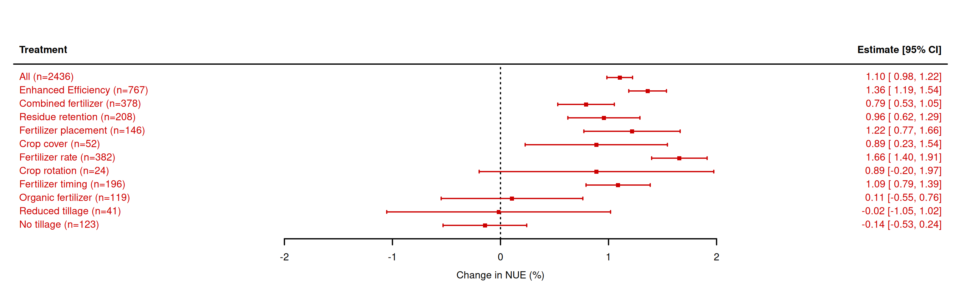
##################################### SMD (metafor) ####################################################
theme_set(theme_bw())

# read data
d1 <- readxl::read_xlsx('Source Data.xlsx',sheet = "Tables")
d1 <- as.data.table(d1)

# Supplement the SD when missing
d2<-d1
CV_nuet_bar<-mean(d2$nuet_sd[is.na(d2$nuet_sd)==FALSE]/d2$nuet_mean[is.na(d2$nuet_sd)==FALSE])
d2$nuet_sd[is.na(d2$nuet_sd)==TRUE]<-d2$nuet_mean[is.na(d2$nuet_sd)==TRUE]*1.25*CV_nuet_bar

CV_nuec_bar<-mean(d2$nuec_sd[is.na(d2$nuec_sd)==FALSE]/d2$nuec_mean[is.na(d2$nuec_sd)==FALSE])
d2$nuec_sd[is.na(d2$nuec_sd)==TRUE]<-d2$nuec_mean[is.na(d2$nuec_sd)==TRUE]*1.25*CV_nuec_bar

# clean up column names
d2 <- as.data.table(d2)
setnames(d2,gsub('\\/','_',gsub(' |\\(|\\)','',colnames(d2))))
setnames(d2,tolower(colnames(d2)))

# calculate effect size (SMD)
es21 <- escalc(measure = "SMD", data = d2, 
               m1i = nuet_mean, sd1i = nuet_sd, n1i = replication,
               m2i = nuec_mean, sd2i = nuec_sd, n2i = replication )

# convert to data.tables
d02 <- as.data.table(es21)

# what are the treatments to be assessed
d02.treat <- data.table(treatment =  c('ALL',unique(d02$management)))

# what are labels
d02.treat[treatment=='ALL',desc := 'All']
d02.treat[treatment=='EE',desc := 'Enhanced Efficiency']
d02.treat[treatment=='CF',desc := 'Combined fertilizer']
d02.treat[treatment=='RES',desc := 'Residue retention']
d02.treat[treatment=='RFP',desc := 'Fertilizer placement']
d02.treat[treatment=='RFR',desc := 'Fertilizer rate']
d02.treat[treatment=='ROT',desc := 'Crop rotation']
d02.treat[treatment=='RFT',desc := 'Fertilizer timing']
d02.treat[treatment=='OF',desc := 'Organic fertilizer']
d02.treat[treatment=='RT',desc := 'Reduced tillage']
d02.treat[treatment=='NT',desc := 'No tillage']
d02.treat[treatment=='CC',desc := 'Crop cover']

# a list to store the coefficients
out2 = out3 = list()

# make a for loop to do a main analysis per treatment
for(i in d02.treat$treatment){
  
  if(i=='ALL'){
    
    # run without selection to estimate overall mean
    r_nue <- rma.mv(yi,vi, data=d02,random= list(~ 1|studyid), method="REML",sparse = TRUE)
    
  } else {
    
    # run for selected treatment
    r_nue <- rma.mv(yi,vi, data=d02[management==i,],random= list(~ 1|studyid), method="REML",sparse = TRUE)
    
  }
  
  # save output in a list
  out2[[i]] <- data.table(mean = as.numeric(r_nue$b),
                          se = as.numeric(r_nue$se),
                          label =  paste0(d02.treat[treatment==i,desc],' (n=',r_nue$k,')')
  )
}

# convert lists to vector
out2 <- rbindlist(out2)

# plot for NUE
forest(x = out2$mean,
       sei = out2$se, slab=out2$label, psize=0.9, cex=1, sortvar=out2$label, xlab="Change in NUE (%)", header="Treatment", col="#CC0000", lwd=2)

Warning in plot.window(...): "sortvar" is not a graphical parameter

Warning in plot.xy(xy, type, ...): "sortvar" is not a graphical parameter

Warning in axis(side = side, at = at, labels = labels, ...): "sortvar" is not a
graphical parameter
Warning in axis(side = side, at = at, labels = labels, ...): "sortvar" is not a
graphical parameter

Warning in box(...): "sortvar" is not a graphical parameter

Warning in title(...): "sortvar" is not a graphical parameter

Warning in int_abline(a = a, b = b, h = h, v = v, untf = untf, ...): "sortvar"
is not a graphical parameter

Warning in segments(...): "sortvar" is not a graphical parameter

Warning in axis(...): "sortvar" is not a graphical parameter

Warning in mtext(...): "sortvar" is not a graphical parameter

Warning in segments(...): "sortvar" is not a graphical parameter
Warning in segments(...): "sortvar" is not a graphical parameter
Warning in segments(...): "sortvar" is not a graphical parameter
Warning in segments(...): "sortvar" is not a graphical parameter
Warning in segments(...): "sortvar" is not a graphical parameter
Warning in segments(...): "sortvar" is not a graphical parameter
Warning in segments(...): "sortvar" is not a graphical parameter
Warning in segments(...): "sortvar" is not a graphical parameter
Warning in segments(...): "sortvar" is not a graphical parameter
Warning in segments(...): "sortvar" is not a graphical parameter
Warning in segments(...): "sortvar" is not a graphical parameter
Warning in segments(...): "sortvar" is not a graphical parameter
Warning in segments(...): "sortvar" is not a graphical parameter
Warning in segments(...): "sortvar" is not a graphical parameter
Warning in segments(...): "sortvar" is not a graphical parameter
Warning in segments(...): "sortvar" is not a graphical parameter
Warning in segments(...): "sortvar" is not a graphical parameter
Warning in segments(...): "sortvar" is not a graphical parameter
Warning in segments(...): "sortvar" is not a graphical parameter
Warning in segments(...): "sortvar" is not a graphical parameter
Warning in segments(...): "sortvar" is not a graphical parameter
Warning in segments(...): "sortvar" is not a graphical parameter
Warning in segments(...): "sortvar" is not a graphical parameter
Warning in segments(...): "sortvar" is not a graphical parameter
Warning in segments(...): "sortvar" is not a graphical parameter
Warning in segments(...): "sortvar" is not a graphical parameter
Warning in segments(...): "sortvar" is not a graphical parameter
Warning in segments(...): "sortvar" is not a graphical parameter
Warning in segments(...): "sortvar" is not a graphical parameter
Warning in segments(...): "sortvar" is not a graphical parameter
Warning in segments(...): "sortvar" is not a graphical parameter
Warning in segments(...): "sortvar" is not a graphical parameter
Warning in segments(...): "sortvar" is not a graphical parameter
Warning in segments(...): "sortvar" is not a graphical parameter
Warning in segments(...): "sortvar" is not a graphical parameter
Warning in segments(...): "sortvar" is not a graphical parameter

Warning in text.default(...): "sortvar" is not a graphical parameter
Warning in text.default(...): "sortvar" is not a graphical parameter

Warning in plot.xy(xy.coords(x, y), type = type, ...): "sortvar" is not a
graphical parameter
Warning in plot.xy(xy.coords(x, y), type = type, ...): "sortvar" is not a
graphical parameter
Warning in plot.xy(xy.coords(x, y), type = type, ...): "sortvar" is not a
graphical parameter
Warning in plot.xy(xy.coords(x, y), type = type, ...): "sortvar" is not a
graphical parameter
Warning in plot.xy(xy.coords(x, y), type = type, ...): "sortvar" is not a
graphical parameter
Warning in plot.xy(xy.coords(x, y), type = type, ...): "sortvar" is not a
graphical parameter
Warning in plot.xy(xy.coords(x, y), type = type, ...): "sortvar" is not a
graphical parameter
Warning in plot.xy(xy.coords(x, y), type = type, ...): "sortvar" is not a
graphical parameter
Warning in plot.xy(xy.coords(x, y), type = type, ...): "sortvar" is not a
graphical parameter
Warning in plot.xy(xy.coords(x, y), type = type, ...): "sortvar" is not a
graphical parameter
Warning in plot.xy(xy.coords(x, y), type = type, ...): "sortvar" is not a
graphical parameter
Warning in plot.xy(xy.coords(x, y), type = type, ...): "sortvar" is not a
graphical parameter

Warning in text.default(...): "sortvar" is not a graphical parameter
Warning in text.default(...): "sortvar" is not a graphical parameter

#publication bias test

#begg’s test
ranktest(out2$mean, out2$se)

Rank Correlation Test for Funnel Plot Asymmetry

Kendall's tau = -0.3939, p = 0.0863

#egger’s test
regtest(out2$mean, out2$se)

Regression Test for Funnel Plot Asymmetry

Model:     mixed-effects meta-regression model
Predictor: standard error

Test for Funnel Plot Asymmetry: z = -1.9366, p = 0.0528
Limit Estimate (as sei -> 0):   b =  1.7600 (CI: 0.9174, 2.6026)

# Meta-regression for main factors

# do a first main factor analysis for log response ratio for NUE

# update the missing values for n_dose and p2o5_dose (as example)
d02[is.na(n_dose), n_dose := median(d02$n_dose,na.rm=TRUE)]

# scale the variables to unit variance
d02[,clay_scaled := scale(clay)]
d02[,soc_scaled := scale(soc)]
d02[,ph_scaled := scale(ph)]
d02[,mat_scaled := scale(mat)]
d02[,map_scaled := scale(map)]
d02[,n_dose_scaled := scale(n_dose)]

# what are the factors to be evaluated
var.site <- c('mat_scaled','map_scaled','clay_scaled','soc_scaled','ph_scaled')
var.crop <- c('g_crop_type','n_dose_scaled')
var.trea <- c('fertilizer_type', 'crop_residue', 'tillage', 'cover_crop_and_crop_rotation', 'fertilizer_strategy')

# i select only one example

# the columns to be assessed
var.sel <- c(var.trea,var.crop,var.site)

# run without a main factor selection to estimate overall mean
r_nue_0 <- rma.mv(yi,vi, data = d02,random= list(~ 1|studyid), method="REML",sparse = TRUE)

# objects to store the effects per factor as wel summary stats of the meta-analytical models
out1.est = out1.sum = list()

# evaluate the impact of treatment (column tillage) on NUE given site properties
for(i in var.sel){
  
  # check whether the column is a numeric or categorical variable
  vartype = is.character(d02[,get(i)])
  
  # run with the main factor treatment
  if(vartype == TRUE){
    
    # run a meta-regression model for main categorial variable
    r_nue_1 <- rma.mv(yi,vi, 
                      mods = ~factor(varsel)-1, 
                      data = d02[,.(yi,vi,studyid,varsel = get(i))],
                      random = list(~ 1|studyid), method="REML",sparse = TRUE)
    
  } else {
    
    # run a meta-regression model for main numerical variable
    r_nue_1 <- rma.mv(yi,vi, 
                      mods = ~varsel, 
                      data = d02[,.(yi,vi,studyid,varsel = get(i))],
                      random = list(~ 1|studyid), method="REML",sparse = TRUE)
  }
  
  # save output in a list: the estimated impact of the explanatory variable
  out1.est[[i]] <- data.table(var = i,
                              varname = gsub('factor\\(varsel\\)','',rownames(r_nue_1$b)),
                              mean = round(as.numeric(r_nue_1$b),3),
                              se = round(as.numeric(r_nue_1$se),3),
                              ci.lb = round(as.numeric(r_nue_1$ci.lb),3),
                              ci.ub = round(as.numeric(r_nue_1$ci.ub),3),
                              pval = round(as.numeric(r_nue_1$pval),3))
  
  # save output in a list: the summary stats collected
  out1.sum[[i]] <- data.table(var = i,
                              AIC = r_nue_1$fit.stats[4,2],
                              ll = r_nue_1$fit.stats[1,2],
                              ll_impr = round(100 * (1-r_nue_1$fit.stats[1,2]/r_nue_0$fit.stats[1,2]),2),
                              r2_impr = round(100*max(0,(sum(r_nue_0$sigma2)-sum(r_nue_1$sigma2))/sum(r_nue_0$sigma2)),2),
                              pval = round(anova(r_nue_1,r_nue_0)$pval,3)
  )
  
}

Warning: REML comparisons not meaningful for models with different fixed effects
(use 'refit=TRUE' to refit both models based on ML estimation).

Warning: REML comparisons not meaningful for models with different fixed effects
(use 'refit=TRUE' to refit both models based on ML estimation).
Warning: REML comparisons not meaningful for models with different fixed effects
(use 'refit=TRUE' to refit both models based on ML estimation).
Warning: REML comparisons not meaningful for models with different fixed effects
(use 'refit=TRUE' to refit both models based on ML estimation).
Warning: REML comparisons not meaningful for models with different fixed effects
(use 'refit=TRUE' to refit both models based on ML estimation).
Warning: REML comparisons not meaningful for models with different fixed effects
(use 'refit=TRUE' to refit both models based on ML estimation).
Warning: REML comparisons not meaningful for models with different fixed effects
(use 'refit=TRUE' to refit both models based on ML estimation).
Warning: REML comparisons not meaningful for models with different fixed effects
(use 'refit=TRUE' to refit both models based on ML estimation).
Warning: REML comparisons not meaningful for models with different fixed effects
(use 'refit=TRUE' to refit both models based on ML estimation).
Warning: REML comparisons not meaningful for models with different fixed effects
(use 'refit=TRUE' to refit both models based on ML estimation).
Warning: REML comparisons not meaningful for models with different fixed effects
(use 'refit=TRUE' to refit both models based on ML estimation).
Warning: REML comparisons not meaningful for models with different fixed effects
(use 'refit=TRUE' to refit both models based on ML estimation).

# merge output into a data.table
out1.sum <- rbindlist(out1.sum)
out1.est <- rbindlist(out1.est)

# Meta-regression for main factors with interactions

# make a function to extract relevant model statistics
estats <- function(model_new,model_base){
  out <- data.table(AIC = model_new$fit.stats[4,2],
                    
                    ll = model_new$fit.stats[1,2],
                    ll_impr = round(100 * (1-model_new$fit.stats[1,2]/model_base$fit.stats[1,2]),2),
                    r2_impr = round(100*max(0,(sum(model_base$sigma2)-sum(model_new$sigma2))/sum(model_base$sigma2)),2),
                    pval = round(anova(r_nue_1,r_nue_0)$pval,3))
  return(out)
}

# update the database

d02[tillage=='reduced', tillage := 'no-till']

d02[,fertilizer_type := factor(fertilizer_type,
                               levels = c('mineral','organic', 'combined','enhanced'))] 
d02[,fertilizer_strategy := factor(fertilizer_strategy,
                                   levels = c("conventional", "placement","rate","timing"))]
d02[,g_crop_type := factor(g_crop_type,
                           levels = c('maize','wheat','rice'))]

d4 <- copy(d02)

d4[,r4pl := fifelse(fertilizer_strategy=='placement','yes','no')]
d4[,r4ti := fifelse(fertilizer_strategy=='timing','yes','no')]
d4[,r4do := fifelse(fertilizer_strategy=='rate','yes','no')]
d4[,ctm := fifelse(g_crop_type=='maize','yes','no')]
d4[,ctw := fifelse(g_crop_type=='wheat','yes','no')]
d4[,ctr := fifelse(g_crop_type=='rice','yes','no')]
d4[,ndose2 := scale(n_dose^2)]

# run without a main factor selection to estimate overall mean
r_nue_0 <- rma.mv(yi,vi, data = d02,random= list(~ 1|studyid), method="REML",sparse = TRUE)

r_nue_4 <- rma.mv(yi,vi,
                  mods = ~fertilizer_type + r4pl + r4ti + r4do + crop_residue + tillage +
                    cover_crop_and_crop_rotation + n_dose_scaled + clay_scaled + ph_scaled + map_scaled + mat_scaled + soc_scaled +
                    soc_scaled : n_dose_scaled + ctm:r4pl + ctm + ctw + ctr + ctm:mat_scaled  + ndose2 -1,
                  data = d4,
                  random = list(~ 1|studyid), method="REML",sparse = TRUE)

Warning: Redundant predictors dropped from the model.

# show stats and improvements
out = estats(model_new = r_nue_4,model_base = r_nue_0)

Warning: REML comparisons not meaningful for models with different fixed effects
(use 'refit=TRUE' to refit both models based on ML estimation).

print(paste0('model improved the log likelyhood with ',round(out$ll_impr,1),'%'))

[1] "model improved the log likelyhood with 3.4%"

summary(r_nue_4)

Multivariate Meta-Analysis Model (k = 2436; method: REML)

    logLik    Deviance         AIC         BIC        AICc   
-4540.2383   9080.4766   9126.4766   9259.6245   9126.9385   

Variance Components:

            estim    sqrt  nlvls  fixed   factor 
sigma^2    1.0930  1.0455    408     no  studyid 

Test for Residual Heterogeneity:
QE(df = 2414) = 6108.4841, p-val < .0001

Test of Moderators (coefficients 1:22):
QM(df = 22) = 616.7506, p-val < .0001

Model Results:

                                 estimate      se     zval    pval    ci.lb 
fertilizer_typemineral             0.4063  0.1183   3.4346  0.0006   0.1744 
fertilizer_typeorganic             0.2806  0.1583   1.7722  0.0764  -0.0297 
fertilizer_typecombined            1.0177  0.1230   8.2745  <.0001   0.7766 
fertilizer_typeenhanced            1.2334  0.1013  12.1774  <.0001   1.0349 
r4plyes                            0.9990  0.1583   6.3106  <.0001   0.6887 
r4tiyes                            0.6162  0.1253   4.9181  <.0001   0.3707 
r4doyes                            0.9923  0.0998   9.9440  <.0001   0.7967 
crop_residueyes                    0.3111  0.1154   2.6968  0.0070   0.0850 
tillageno-till                    -0.4592  0.1193  -3.8503  0.0001  -0.6929 
cover_crop_and_crop_rotationyes    0.4683  0.2082   2.2490  0.0245   0.0602 
n_dose_scaled                     -0.1746  0.1246  -1.4015  0.1611  -0.4187 
clay_scaled                       -0.1196  0.0563  -2.1246  0.0336  -0.2299 
ph_scaled                          0.0579  0.0809   0.7155  0.4743  -0.1007 
map_scaled                         0.1446  0.0912   1.5863  0.1127  -0.0341 
mat_scaled                        -0.1060  0.0782  -1.3562  0.1750  -0.2592 
soc_scaled                        -0.0032  0.0638  -0.0509  0.9594  -0.1283 
ctmyes                             0.0563  0.1181   0.4773  0.6332  -0.1750 
ctwyes                            -0.0199  0.1039  -0.1911  0.8484  -0.2236 
ndose2                             0.1757  0.1154   1.5228  0.1278  -0.0504 
n_dose_scaled:soc_scaled          -0.0208  0.0309  -0.6736  0.5006  -0.0814 
r4plyes:ctmyes                    -0.7457  0.2588  -2.8810  0.0040  -1.2530 
mat_scaled:ctmyes                  0.1425  0.1149   1.2406  0.2147  -0.0826 
                                   ci.ub      
fertilizer_typemineral            0.6382  *** 
fertilizer_typeorganic            0.5909    . 
fertilizer_typecombined           1.2587  *** 
fertilizer_typeenhanced           1.4319  *** 
r4plyes                           1.3093  *** 
r4tiyes                           0.8618  *** 
r4doyes                           1.1879  *** 
crop_residueyes                   0.5372   ** 
tillageno-till                   -0.2254  *** 
cover_crop_and_crop_rotationyes   0.8764    * 
n_dose_scaled                     0.0696      
clay_scaled                      -0.0093    * 
ph_scaled                         0.2165      
map_scaled                        0.3233      
mat_scaled                        0.0472      
soc_scaled                        0.1218      
ctmyes                            0.2877      
ctwyes                            0.1838      
ndose2                            0.4018      
n_dose_scaled:soc_scaled          0.0397      
r4plyes:ctmyes                   -0.2384   ** 
mat_scaled:ctmyes                 0.3676      

---
Signif. codes:  0 '***' 0.001 '**' 0.01 '*' 0.05 '.' 0.1 ' ' 1

k <- r_nue_4$k
wi <- 1/r_nue_4$vi
vt <- (k-1) / (sum(wi) - sum(wi^2)/sum(wi))
PR2 <- r_nue_0$sigma2 / (sum(r_nue_4$sigma2) + vt)


#######################################meta of meta-analytical data###########################################################

#Load libraries 
library(ggplot2)
library(dplyr)

Attaching package: 'dplyr'

The following objects are masked from 'package:data.table':

    between, first, last

The following objects are masked from 'package:stats':

    filter, lag

The following objects are masked from 'package:base':

    intersect, setdiff, setequal, union

library(gridExtra)

Attaching package: 'gridExtra'

The following object is masked from 'package:dplyr':

    combine

library(cowplot)
library(openxlsx)
library(gg.gap)
library(ggforce)
library(data.table)

malit <- readxl::read_xlsx('Source Data.xlsx',sheet = "meta_of_meta-analytica_data")
malit <- as.data.table(malit)

# create subset of columns we need (later subselection to match the df2)

df <- data.frame(reference=malit$reference, ind_code=malit$ind_code, man_code=malit$man_code, 
                 man=malit$man, ind=malit$ind, man_type=malit$man_type, type.m=as.character(malit$type.m), n.S=1, 
                 dyr.1=malit$dyr.1, SEyr.1=as.numeric(malit$Seyr.1),unit=malit$unit, n.O=malit$n)

# weighted mean

df1 <- df %>% group_by(ind_code,man_code,ind,man) %>% 
  summarise(type.m= "Weighted mean", dyr.1 = weighted.mean(dyr.1, 1/SEyr.1),
            reference = paste0(reference, collapse = ", "), n.S = n(), n.O = sum(n.O), man_type=first(man_type))

`summarise()` has grouped output by 'ind_code', 'man_code', 'ind'. You can
override using the `.groups` argument.

df1 <-data.frame(df1)
# weighted mean SE MIN
df2 <- df %>% group_by(ind_code,man_code,ind,man) %>% 
  summarise(type.m= "Weighted mean SE", dyr.1 = (weighted.mean(dyr.1, 1/SEyr.1)-(1/sqrt(sum(1/SEyr.1)))),
            reference = paste0(reference, collapse = ", "), n.S = n(), n.O = sum(n.O), man_type=first(man_type))

`summarise()` has grouped output by 'ind_code', 'man_code', 'ind'. You can
override using the `.groups` argument.

df2 <-data.frame(df2)

# weighted mean SE Max
df3 <- df %>% group_by(ind_code,man_code,ind,man) %>% 
  summarise(type.m= "Weighted mean SE", dyr.1 = weighted.mean(dyr.1, 1/SEyr.1)+(1/sqrt(sum(1/SEyr.1))),
            reference = paste0(reference, collapse = ", "), n.S = n(), n.O = sum(n.O), man_type=first(man_type))

`summarise()` has grouped output by 'ind_code', 'man_code', 'ind'. You can
override using the `.groups` argument.

df3 <-data.frame(df3)

# SE MIN
df4 <- df %>% group_by(ind_code,man_code,ind,man) %>% 
  summarise(type.m= "Min and max SE", dyr.1 = min(dyr.1-SEyr.1),
            reference = paste0(reference, collapse = ", "), n.S = n(), n.O = sum(n.O), man_type=first(man_type))

`summarise()` has grouped output by 'ind_code', 'man_code', 'ind'. You can
override using the `.groups` argument.

df4 <-data.frame(df4)

# SE MAX
df5 <- df %>% group_by(ind_code,man_code,ind,man) %>% 
  summarise(type.m= "Min and max SE", dyr.1 = max(dyr.1+SEyr.1),
            reference = paste0(reference, collapse = ", "), n.S = n(), n.O = sum(n.O), man_type=first(man_type))

`summarise()` has grouped output by 'ind_code', 'man_code', 'ind'. You can
override using the `.groups` argument.

df5 <-data.frame(df5)

# find min and max individual means to write to output file
df_range <- df %>% group_by(ind_code,man_code,ind,man) %>% 
  summarise(min_im = min(dyr.1), max_im = max(dyr.1))

`summarise()` has grouped output by 'ind_code', 'man_code', 'ind'. You can
override using the `.groups` argument.

# make a data frame with data we need from individual means with same column names
df_im <- data.frame(reference=df$reference, ind_code=df$ind_code, man_code=df$man_code, ind=df$ind, man=df$man,
                    man_type=malit$man_type, type.m=df$type.m, dyr.1=df$dyr.1, n.S=df$n.S, n.O=df$n.O)



# use rbind to combine 
df_wm <- rbind(df_im, df1, df2, df3, df4, df5)
df_means <- subset(df_wm, type.m=="Weighted mean")

df_means <- data.frame(indicator=df_means$ind, management=df_means$man, man_type=df_means$man_type, 
                       wm = signif(df_means$dyr.1, digits=2))
df_means <- cbind(df_means, min_im = df_range$min_im, max_im = df_range$max_im)

df_wm$man <- factor(as.factor(df_wm$man), levels=c("Enhanced efficiency (A)",
                                                   "Fertilizer placement (4R)",
                                                   "Fertilizer timing (4R)",
                                                   "Fertilizer rate (4R)",
                                                   "Combined fertilizer (4R)",
                                                   "Organic fertilizer (4R)",
                                                   "No tillage (T)",
                                                   "Reduced tillage (T)",
                                                   "Residue retention (C)",
                                                   "Cover cropping (C)",
                                                   "Crop rotation (C)"))

df_means

   indicator                management man_type    wm   min_im   max_im
1        NUE        Cover cropping (C)        C -13.0 -35.9113 19.00000
2        NUE  Combined fertilizer (4R)       4R   1.9 -27.1000 32.81440
3        NUE   Enhanced efficiency (A)        A  14.0 -13.7438 57.39500
4        NUE            No tillage (T)        T  -2.3 -16.9400 29.70440
5        NUE   Organic fertilizer (4R)       4R  -1.1 -43.0049 71.22417
6        NUE     Residue retention (C)        C   6.9  -1.0000 36.00000
7        NUE Fertilizer placement (4R)       4R  28.0  25.2000 31.47780
8        NUE      Fertilizer rate (4R)       4R  17.0 -18.1773 82.51748
9        NUE    Fertilizer timing (4R)       4R   6.7 -18.1773 42.48000
10       NUE         Crop rotation (C)        C  38.0  38.0000 38.00000
11       NUE       Reduced tillage (T)        T  -9.0  -9.0000 -9.00000

# write.xlsx(df_means, file="data/meta of meta-analytical results.xlsx", sheetName = "Weighted mean results", colNames = TRUE, rowNames = TRUE, append = FALSE)